
Signals and Systems
Collection edited by: Richard Baraniuk
Content authors: Melissa Selik, Richard Baraniuk, Michael Haag, Stephen Kruzick, Don Johnson, Dan Calderon, Thanos Antoulas, John Slavinsky, Dante Soares, Justin Romberg, Ricardo Radaelli-Sanchez, Catherine Elder, Benjamin Fite, Roy Ha, C. Burrus, Steven Cox, and Matthew Hutchinson
Online: <http://cnx.org/content/col10064/1.14>
This selection and arrangement of content as a collection is copyrighted by Richard Baraniuk.
It is licensed under the Creative Commons Attribution License: http://creativecommons.org/licenses/by/3.0/
Collection structure revised: 2011/10/11
For copyright and attribution information for the modules contained in this collection, see the "Attributions" section at the end of the collection.
Signals and Systems
Table of Contents
3. Time Domain Analysis of Continuous Time Systems
4. Time Domain Analysis of Discrete Time Systems
5. Introduction to Fourier Analysis
6. Continuous Time Fourier Series (CTFS)
7. Discrete Time Fourier Series (DTFS)
8. Continuous Time Fourier Transform (CTFT)
9. Discrete Time Fourier Transform (DTFT)
10. Sampling and Reconstruction
11. Laplace Transform and Continuous Time System Design
12. Z-Transform and Discrete Time System Design
13. Capstone Signal Processing Topics
14. Appendix A: Linear Algebra Overview
15. Appendix B: Hilbert Spaces Overview
16. Appendix C: Analysis Topics Overview
17. Appendix D: Viewing Interactive Content
Signals and Systems
Collection edited by: Richard Baraniuk
Content authors: Melissa Selik, Richard Baraniuk, Michael Haag, Stephen Kruzick, Don Johnson, Dan Calderon, Thanos Antoulas, John Slavinsky, Dante Soares, Justin Romberg, Ricardo Radaelli-Sanchez, Catherine Elder, Benjamin Fite, Roy Ha, C. Burrus, Steven Cox, and Matthew Hutchinson
Online: <http://cnx.org/content/col10064/1.14>
This selection and arrangement of content as a collection is copyrighted by Richard Baraniuk.
It is licensed under the Creative Commons Attribution License: http://creativecommons.org/licenses/by/3.0/
Collection structure revised: 2011/10/11
For copyright and attribution information for the modules contained in this collection, see the "Attributions" section at the end of the collection.
Chapter 1. Introduction to Signals
1.1. Signal Classifications and Properties*
Introduction
This module will begin our study of signals and systems by laying out some of the fundamentals of signal classification. It is essentially an introduction to the important definitions and properties that are fundamental to the discussion of signals and systems, with a brief discussion of each.
Classifications of Signals
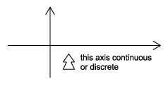
Continuous-Time vs. Discrete-Time
As the names suggest, this classification is determined by whether or not the time axis is discrete (countable) or continuous (Figure 1.1). A continuous-time signal will contain a value for all real numbers along the time axis. In contrast to this, a discrete-time signal, often created by sampling a continuous signal, will only have values at equally spaced intervals along the time axis.
Figure 1.1.
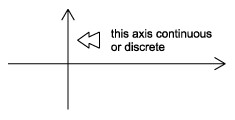
Analog vs. Digital
The difference between analog and digital is similar to the difference between continuous-time and discrete-time. However, in this case the difference involves the values of the function. Analog corresponds to a continuous set of possible function values, while digital corresponds to a discrete set of possible function values. An common example of a digital signal is a binary sequence, where the values of the function can only be one or zero.
Figure 1.2.
Periodic vs. Aperiodic
Periodic signals repeat with some period T , while aperiodic, or nonperiodic, signals do not (Figure 1.3). We can define a periodic function through the following mathematical expression, where t can be any number and T is a positive constant: f(t) = f(T + t) The fundamental period of our function, f(t) , is the smallest value of T that the still allows Equation to be true.
Figure 1.3.

(a) A periodic signal with period T 0

(b) An aperiodic signal
Finite vs. Infinite Length
As the name implies, signals can be characterized as to whether they have a finite or infinite length set of values. Most finite length signals are used when dealing with discrete-time signals or a given sequence of values. Mathematically speaking, f(t) is a finite-length signal if it is nonzero over a finite interval t 1 < f(t) < t 2 where t 1 > – ∞ and t 2 < ∞ . An example can be seen in Figure 1.4. Similarly, an infinite-length signal, f(t) , is defined as nonzero over all real numbers: ∞ ≤ f(t) ≤ – ∞
Figure 1.4.

Finite-Length Signal. Note that it only has nonzero values on a set, finite interval.
Causal vs. Anticausal vs. Noncausal
Causal signals are signals that are zero for all negative time, while anticausal are signals that are zero for all positive time. Noncausal signals are signals that have nonzero values in both positive and negative time (Figure 1.5).
Figure 1.5.
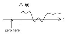
(a) A causal signal
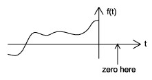
(b) An anticausal signal
(c) A noncausal signal
Even vs. Odd
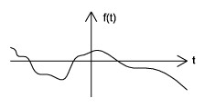
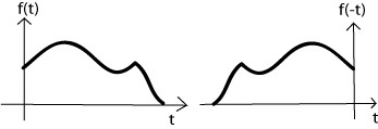
An even signal is any signal f such that f(t) = f( – t) . Even signals can be easily spotted as they are symmetric around the vertical axis. An odd signal, on the other hand, is a signal f such that f(t) = – (f( – t)) (Figure 1.6).
Figure 1.6.
(a) An even signal
(b) An odd signal
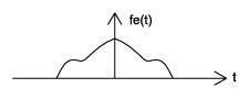
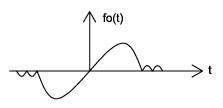
Using the definitions of even and odd signals, we can show that any signal can be written as a combination of an even and odd signal. That is, every signal has an odd-even decomposition. To demonstrate this, we have to look no further than a single equation. 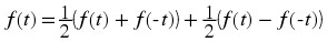 By multiplying and adding this expression out, it can be shown to be true. Also, it can be shown that f(t) + f( – t) fulfills the requirement of an even function, while f(t) − f( – t) fulfills the requirement of an odd function (Figure 1.7).
Example 1.1.
Figure 1.7.
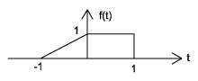
(a) The signal we will decompose using odd-even decomposition
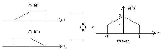
(b) Even part:
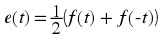
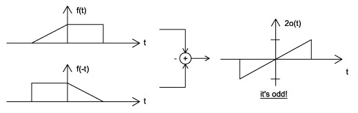
(c) Odd part:
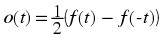
(d) Check: e(t) + o(t) = f(t)
Deterministic vs. Random
A deterministic signal is a signal in which each value of the signal is fixed and can be determined by a mathematical expression, rule, or table. Because of this the future values of the signal can be calculated from past values with complete confidence. On the other hand, a random signal has a lot of uncertainty about its behavior. The future values of a random signal cannot be accurately predicted and can usually only be guessed based on the averages of sets of signals (Figure 1.8).
Figure 1.8.
(a) Deterministic Signal
(b) Random Signal
Example 1.2.
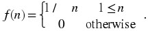
Consider the signal defined for all real t described by
(1.1)
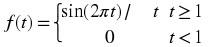
This signal is continuous time, analog, aperiodic, infinite length, causal, neither even nor odd, and, by definition, deterministic.
Signal Classifications Summary
This module describes just some of the many ways in which signals can be classified. They can be continuous time or discrete time, analog or digital, periodic or aperiodic, finite or infinite, and deterministic or random. We can also divide them based on their causality and symmetry properties. There are other ways to classify signals, such as boundedness, handedness, and continuity, that are not discussed here but will be described in subsequent modules.
1.2. Signal Size and Norms*
Introduction
The "size" of a signal would involve some notion of its strength. We use the mathematical concept of the norm to quantify this concept for both continuous-time and discrete-time signals. As there are several types of norms that can be defined for signals, there are several different conceptions of signal size.
Signal Energy
Infinite Length, Continuous Time Signals
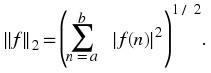
The most commonly encountered notion of the energy of a signal defined on R is the L 2 norm defined by the square root of the integral of the square of the signal, for which the notation
(1.2) | | f | | 2 = (∫∞ – ∞ | f ( t ) | 2 d t) 1 / 2 .
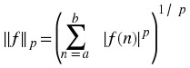
However, this idea can be generalized through definition of the L p norm, which is given by
(1.3) | | f | | p = (∫∞ – ∞ | f ( t ) | p d t) 1 / p
for all 1 ≤ p < ∞. Because of the behavior of this expression as p approaches ∞, we furthermore define
(1.4)
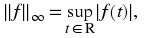
which is the least upper bound of |f(t)|. A signal f is said to belong to the vector space L p (R) if ||f||p < ∞.
Example 1.3.
For example, consider the function defined by
(1.5)
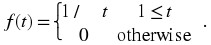
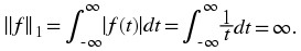
The L 1 norm is
(1.6)
The L 2 norm is
(1.7)
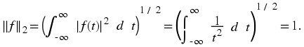
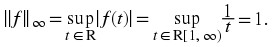
The L ∞ norm is
(1.8)
Finite Length, Continuous Time Signals
The most commonly encountered notion of the energy of a signal defined on R[a,b] is the L 2 norm defined by the square root of the integral of the square of the signal, for which the notation
(1.9) | | f | | 2 = (∫b a | f ( t ) | 2 d t) 1 / 2 .
However, this idea can be generalized through definition of the L p norm, which is given by
(1.10) | | f | | p = (∫b a | f ( t ) | p d t) 1 / p
for all 1 ≤ p < ∞. Because of the behavior of this expression as p approaches ∞, we furthermore define
(1.11)
which is the least upper bound of |f(t)|. A signal f is said to belong to the vector space L p (R[a,b]) if ||f||p < ∞. The periodic extension of such a signal would have infinite energy but finite power.
Example 1.4.
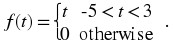
For example, consider the function defined on R[ – 5,3] by
(1.12)
The L 1 norm is
(1.13) | | f | | 1 = ∫3 – 5 | f ( t ) | d t = ∫3 – 5 | t | d t = 17 .
The L 2 norm is
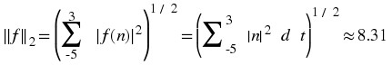
(1.14) | | f | | 2 = (∫3 – 5 | f ( t ) | 2 d t) 1 / 2 = (∫3 – 5 | t | 2 d t) 1 / 2 ≈ 7 . 12
The L ∞ norm is
(1.15)
Infinite Length, Discrete Time Signals
The most commonly encountered notion of the energy of a signal defined on Z is the l 2 norm defined by the square root of the sumation of the square of the signal, for which the notation
(1.16)
However, this idea can be generalized through definition of the l p norm, which is given by
(1.17)
for all 1 ≤ p < ∞. Because of the behavior of this expression as p approaches ∞, we furthermore define
(1.18)
which is the least upper bound of |f(n)|. A signal f is said to belong to the vector space l p (Z) if ||f||p < ∞.
Example 1.5.
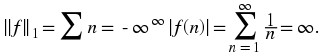
For example, consider the function defined by
(1.19)
The l 1 norm is
(1.20)
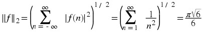
The l 2 norm is
(1.21)
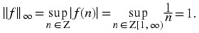
The l ∞ norm is
(1.22)
Finite Length, Discrete Time Signals
The most commonly encountered notion of the energy of a signal defined on Z[a,b] is the l 2 norm defined by the square root of the sumation of the square of the signal, for which the notation
(1.23)
However, this idea can be generalized through definition of the l p norm, which is given by
(1.24)
for all 1 ≤ p < ∞. Because of the behavior of this expression as p approaches ∞, we furthermore define
(1.25)

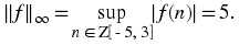
which is the least upper bound of |f(n)|. In this case, this least upper bound is simply the maximum value of |f(n)|. A signal f is said to belong to the vector space l p (Z[a,b]) if ||f||p < ∞. The periodic extension of such a signal would have infinite energy but finite power.
Example 1.6.
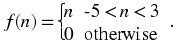
For example, consider the function defined on Z[ – 5,3] by
(1.26)
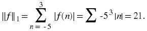
The l 1 norm is
(1.27)
The l 2 norm is
(1.28)
The l ∞ norm is
(1.29)
Signal Norms Summary
The notion of signal size or energy is formally addressed through the mathematical concept of norms. There are many types of norms that can be defined for signals, some of the most important of which have been discussed here. For each type norm and each type of signal domain (continuous or discrete, and finite or infinite) there are vector spaces defined for signals of finite norm. Finally, while nonzero periodic signals have infinite energy, they have finite power if their single period units have finite energy.
1.3. Signal Operations*
Introduction
This module will look at two signal operations affecting the time parameter of the signal, time shifting and time scaling. These operations are very common components to real-world systems and, as such, should be understood thoroughly when learning about signals and systems.
Manipulating the Time Parameter
Time Shifting
Time shifting is, as the name suggests, the shifting of a signal in time. This is done by adding or subtracting a quantity of the shift to the time variable in the function. Subtracting a fixed positive quantity from the time variable will shift the signal to the right (delay) by the subtracted quantity, while adding a fixed positive amount to the time variable will shift the signal to the left (advance) by the added quantity.
Figure 1.9.
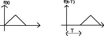
f(t − T) moves (delays) f to the right by T .
Time Scaling
Time scaling compresses or dilates a signal by multiplying the time variable by some quantity. If that quantity is greater than one, the signal becomes narrower and the operation is called compression, while if the quantity is less than one, the signal becomes wider and is called dilation.
Figure 1.10.
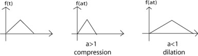
f(at) compresses f by a .
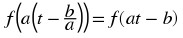
Example 1.7.
Given f(t) we woul like to plot f(a t – b). The figure below describes a method to accomplish this.
Figure 1.11.
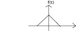
(a) Begin with f(t)
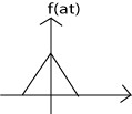
(b) Then replace t with at to get f(at)
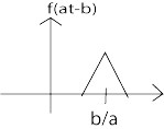
(c) Finally, replace t withto get
Time Reversal
A natural question to consider when learning about time scaling is: What happens when the time variable is multiplied by a negative number? The answer to this is time reversal. This operation is the reversal of the time axis, or flipping the signal over the y-axis.
Figure 1.12.
Reverse the time axis
Time Scaling and Shifting Demonstration
Figure 1.13.
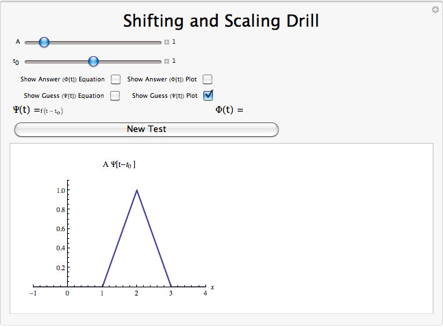
Download or Interact (when online) with a Mathematica CDF demonstrating Discrete Harmonic Sinusoids.
Signal Operations Summary
Some common operations on signals affect the time parameter of the signal. One of these is time shifting in which a quantity is added to the time parameter in order to advance or delay the signal. Another is the time scaling in which the time parameter is multiplied by a quantity in order to dilate or compress the signal in time. In the event that the quantity involved in the latter operation is negative, time reversal occurs.
1.4. Common Continuous Time Signals*
Introduction
Before looking at this module, hopefully you have an idea of what a signal is and what basic classifications and properties a signal can have. In review, a signal is a function defined with respect to an independent variable. This variable is often time but could represent any number of things. Mathematically, continuous time analog signals have continuous independent and dependent variables. This module will describe some useful continuous time analog signals.
Important Continuous Time Signals
Sinusoids
One of the most important elemental signal that you will deal with is the real-valued sinusoid. In its continuous-time form, we write the general expression as Acos(ωt + φ) where A is the amplitude, ω is the frequency, and φ is the phase. Thus, the period of the sinusoid is 
Figure 1.14.
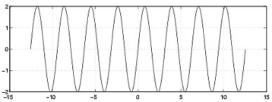
Sinusoid with A = 2 , w = 2 , and φ = 0 .
Complex Exponentials
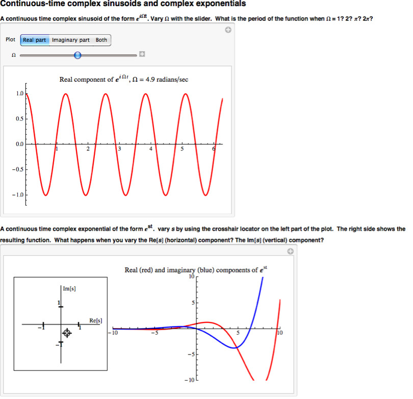
As important as the general sinusoid, the complex exponential function will become a critical part of your study of signals and systems. Its general continuous form is written as A ⅇ st where s = σ + jω is a complex number in terms of σ , the attenuation constant, and ω the angular frequency.
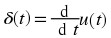
Unit Impulses
The unit impulse function, also known as the Dirac delta function, is a signal that has infinite height and infinitesimal width. However, because of the way it is defined, it integrates to one. While this signal is useful for the understanding of many concepts, a formal understanding of its definition more involved. The unit impulse is commonly denoted δ(t) .
More detail is provided in the section on the continuous time impulse function. For now, it suffices to say that this signal is crucially important in the study of continuous signals, as it allows the sifting property to be used in signal representation and signal decomposition.
Unit Step
Another very basic signal is the unit-step function that is defined as 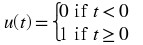
Figure 1.15.
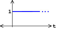
Continuous-Time Unit-Step Function
The step function is a useful tool for testing and for defining other signals. For example, when different shifted versions of the step function are multiplied by other signals, one can select a certain portion of the signal and zero out the rest.
Common Continuous Time Signals Summary
Some of the most important and most frequently encountered signals have been discussed in this module. There are, of course, many other signals of significant consequence not discussed here. As you will see later, many of the other more complicated signals will be studied in terms of those listed here. Especially take note of the complex exponentials and unit impulse functions, which will be the key focus of several topics included in this course.
1.5. Common Discrete Time Signals*
Introduction
Before looking at this module, hopefully you have an idea of what a signal is and what basic classifications and properties a signal can have. In review, a signal is a function defined with respect to an independent variable. This variable is often time but could represent any number of things. Mathematically, discrete time analog signals have discrete independent variables and continuous dependent variables. This module will describe some useful discrete time analog signals.
Important Discrete Time Signals
Sinusoids
One of the most important elemental signal that you will deal with is the real-valued sinusoid. In its discrete-time form, we write the general expression as Acos(ωn + φ) where A is the amplitude, ω is the frequency, and φ is the phase. Because n only takes integer values, the resulting function is only periodic if  is a rational number.
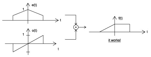
Figure 1.16. Discrete-Time Cosine Signal
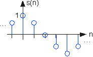
A discrete-time cosine signal is plotted as a stem plot.
Note that the equation representation for a discrete time sinusoid waveform is not unique.
Complex Exponentials
As important as the general sinusoid, the complex exponential function will become a critical part of your study of signals and systems. Its general discrete form is written as A ⅇ sn where s = σ + jω , is a complex number in terms of σ , the attenuation constant, and ω the angular frequency.
The discrete time complex exponentials have the following property. ⅇ jωn = ⅇ j(ω + 2π)n Given this property, if we have a complex exponential with frequency ω + 2π , then this signal "aliases" to a complex exponential with frequency ω , implying that the equation representations of discrete complex exponentials are not unique.
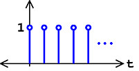
Unit Impulses
The second-most important discrete-time signal is the unit sample, which is defined as 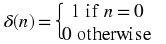
Figure 1.17. Unit Sample

The unit sample.
More detail is provided in the section on the discrete time impulse function. For now, it suffices to say that this signal is crucially important in the study of discrete signals, as it allows the sifting property to be used in signal representation and signal decomposition.
Unit Step
Another very basic signal is the unit-step function defined as 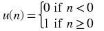
Figure 1.18.
Discrete-Time Unit-Step Function
The step function is a useful tool for testing and for defining other signals. For example, when different shifted versions of the step function are multiplied by other signals, one can select a certain portion of the signal and zero out the rest.
Common Discrete Time Signals Summary
Some of the most important and most frequently encountered signals have been discussed in this module. There are, of course, many other signals of significant consequence not discussed here. As you will see later, many of the other more complicated signals will be studied in terms of those listed here. Especially take note of the complex exponentials and unit impulse functions, which will be the key focus of several topics included in this course.
1.6. Continuous Time Impulse Function*
Introduction
In engineering, we often deal with the idea of an action occurring at a point. Whether it be a force at a point in space or some other signal at a point in time, it becomes worth while to develop some way of quantitatively defining this. This leads us to the idea of a unit impulse, probably the second most important function, next to the complex exponential, in this systems and signals course.
Dirac Delta Function
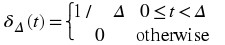
The Dirac delta function, often referred to as the unit impulse or delta function, is the function that defines the idea of a unit impulse in continuous-time. Informally, this function is one that is infinitesimally narrow, infinitely tall, yet integrates to one. Perhaps the simplest way to visualize this is as a rectangular pulse from  to
to  with a height of
  . As we take the limit of this setup as ε approaches 0, we see that the width tends to zero and the height tends to infinity as the total area remains constant at one. The impulse function is often written as δ(t) .
(1.30)

Figure 1.19.
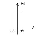
This is one way to visualize the Dirac Delta Function.
Figure 1.20.
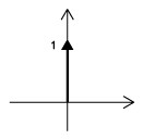
Since it is quite difficult to draw something that is infinitely tall, we represent the Dirac with an arrow centered at the point it is applied. If we wish to scale it, we may write the value it is scaled by next to the point of the arrow. This is a unit impulse (no scaling).
Below is a brief list a few important properties of the unit impulse without going into detail of their proofs.
Unit Impulse Properties
δ(t) = δ( – t)
 , where u(t) is the unit step.
 f ( t ) δ ( t ) = f ( 0 ) δ ( t )
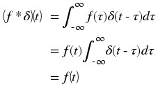
The last of these is especially important as it gives rise to the sifting property of the dirac delta function, which selects the value of a function at a specific time and is especially important in studying the relationship of an operation called convolution to time domain analysis of linear time invariant systems. The sifting property is shown and derived below. ∫∞ – ∞ f ( t ) δ ( t ) d t = ∫∞ – ∞ f ( 0 ) δ ( t ) d t = f ( 0 ) ∫∞ – ∞ δ ( t ) d t = f ( 0 )
Unit Impulse Limiting Demonstration
Figure 1.21.
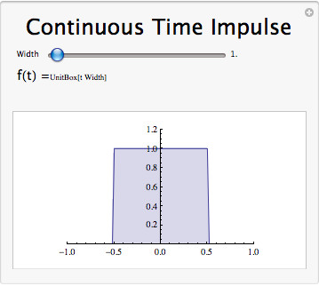
Click on the above thumbnail image (when online) to download an interactive Mathematica Player demonstrating the Continuous Time Impulse Function.
Continuous Time Unit Impulse Summary
The continuous time unit impulse function, also known as the Dirac delta function, is of great importance to the study of signals and systems. Informally, it is a function with infinite height ant infinitesimal width that integrates to one, which can be viewed as the limiting behavior of a unit area rectangle as it narrows while preserving area. It has several important properties that will appear again when studying systems.
1.7. Discrete Time Impulse Function*
Introduction
In engineering, we often deal with the idea of an action occurring at a point. Whether it be a force at a point in space or some other signal at a point in time, it becomes worth while to develop some way of quantitatively defining this. This leads us to the idea of a unit impulse, probably the second most important function, next to the complex exponential, in this systems and signals course.
Unit Sample Function
The unit sample function, often referred to as the unit impulse or delta function, is the function that defines the idea of a unit impulse in discrete time. There are not nearly as many intricacies involved in its definition as there are in the definition of the Dirac delta function, the continuous time impulse function. The unit sample function simply takes a value of one at n=0 and a value of zero elsewhere. The impulse function is often written as δ(n) . 
Figure 1.22. Unit Sample
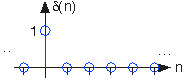
The unit sample.
Below we will briefly list a few important properties of the unit impulse without going into detail of their proofs.
Unit Impulse Properties
δ(n) = δ( – n)
δ ( n ) = u ( n ) – u ( n – 1 )
f ( n ) δ ( n ) = f ( 0 ) δ ( n )
The last of these is especially important as it gives rise to the sifting property of the unit sample function, which selects the value of a function at a specific time and is especially important in studying the relationship of an operation called convolution to time domain analysis of linear time invariant systems. The sifting property is shown and derived below. 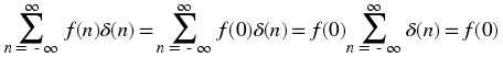
Discrete Time Impulse Response Demonstration
Figure 1.23.
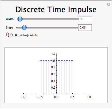
Interact(when online) with a Mathematica CDF demonstrating the Discrete Time Impulse Function.
Discrete Time Unit Impulse Summary
The discrete time unit impulse function, also known as the unit sample function, is of great importance to the study of signals and systems. The function takes a value of one at time n=0 and a value of zero elsewhere. It has several important properties that will appear again when studying systems.
1.8. Continuous Time Complex Exponential*
Introduction
Complex exponentials are some of the most important functions in our study of signals and systems. Their importance stems from their status as eigenfunctions of linear time invariant systems. Before proceeding, you should be familiar with complex numbers.
The Continuous Time Complex Exponential
Complex Exponentials
The complex exponential function will become a critical part of your study of signals and systems. Its general continuous form is written as A ⅇ st where s = σ + ⅈω is a complex number in terms of σ , the attenuation constant, and ω the angular frequency.
Euler's Formula
The mathematician Euler proved an important identity relating complex exponentials to trigonometric functions. Specifically, he discovered the eponymously named identity, Euler's formula, which states that
(1.31)e jx = cos ( x ) + j sin ( x )
which can be proven as follows.
In order to prove Euler's formula, we start by evaluating the Taylor series for e z about z = 0, which converges for all complex z , at z = j x . The result is
(1.32)
because the second expression contains the Taylor series for cos(x) and sin(x) about t = 0, which converge for all real x . Thus, the desired result is proven.
Choosing x = ω t this gives the result
(1.33)e jωt = cos ( ω t ) + j sin ( ω t )
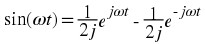
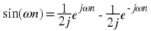
which breaks a continuous time complex exponential into its real part and imaginary part. Using this formula, we can also derive the following relationships.
(1.34)

(1.35)
Continuous Time Phasors
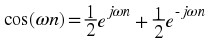
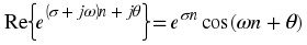
It has been shown how the complex exponential with purely imaginary frequency can be broken up into its real part and its imaginary part. Now consider a general complex frequency s = σ + ω j where σ is the attenuation factor and ω is the frequency. Also consider a phase difference θ . It follows that
(1.36)e ( σ + j ω ) t + j θ = e σt (cos ( ω t + θ ) + j sin ( ω t + θ )) .
Thus, the real and imaginary parts of e st appear below.
(1.37)
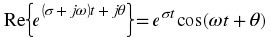
(1.38)
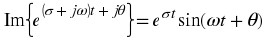
Using the real or imaginary parts of complex exponential to represent sinusoids with a phase delay multiplied by real exponential is often useful and is called attenuated phasor notation.
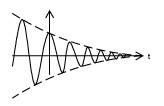
We can see that both the real part and the imaginary part have a sinusoid times a real exponential. We also know that sinusoids oscillate between one and negative one. From this it becomes apparent that the real and imaginary parts of the complex exponential will each oscillate within an envelope defined by the real exponential part.
Figure 1.24.

(a) If σ is negative, we have the case of a decaying exponential window.
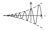
(b) If σ is positive, we have the case of a growing exponential window.
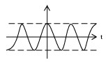
(c) If σ is zero, we have the case of a constant window.
The shapes possible for the real part of a complex exponential. Notice that the oscillations are the result of a cosine, as there is a local maximum at t = 0 .
Complex Exponential Demonstration
Figure 1.25.
Interact (when online) with a Mathematica CDF demonstrating the Continuous Time Complex Exponential. To Download, right-click and save target as .cdf.
Continuous Time Complex Exponential Summary
Continuous time complex exponentials are signals of great importance to the study of signals and systems. They can be related to sinusoids through Euler's formula, which identifies the real and imaginary parts of purely imaginary complex exponentials. Eulers formula reveals that, in general, the real and imaginary parts of complex exponentials are sinusoids multiplied by real exponentials. Thus, attenuated phasor notation is often useful in studying these signals.
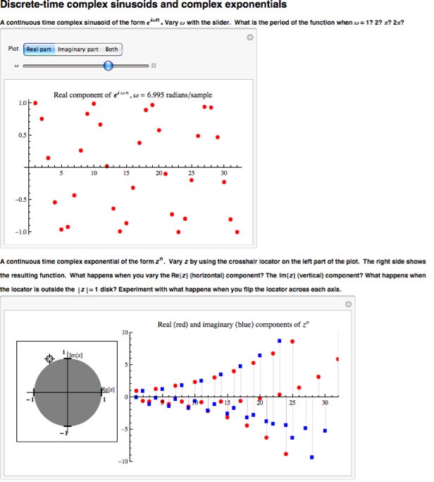
1.9. Discrete Time Complex Exponential*
Introduction
Complex exponentials are some of the most important functions in our study of signals and systems. Their importance stems from their status as eigenfunctions of linear time invariant systems. Before proceeding, you should be familiar with complex numbers.
The Discrete Time Complex Exponential
Complex Exponentials
The complex exponential function will become a critical part of your study of signals and systems. Its general discrete form is written as A ⅇ sn where s = σ + ⅈω , is a complex number in terms of σ , the attenuation constant, and ω the angular frequency.
The discrete time complex exponentials have the following property, which will become evident through discussion of Euler's formula. ⅇ ⅈωn = ⅇ ⅈ(ω + 2π)n Given this property, if we have a complex exponential with frequency ω + 2π , then this signal "aliases" to a complex exponential with frequency ω , implying that the equation representations of discrete complex exponentials are not unique.
Euler's Formula
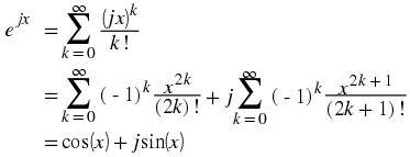
The mathematician Euler proved an important identity relating complex exponentials to trigonometric functions. Specifically, he discovered the eponymously named identity, Euler's formula, which states that
(1.39)e jx = cos ( x ) + j sin ( x )
which can be proven as follows.
In order to prove Euler's formula, we start by evaluating the Taylor series for e z about z = 0, which converges for all complex z , at z = j x . The result is
(1.40)

because the second expression contains the Taylor series for cos(x) and sin(x) about t = 0, which converge for all real x . Thus, the desired result is proven.
Choosing x = ω n this gives the result
(1.41)e jωn = cos ( ω n ) + j sin ( ω n )
which breaks a discrete time complex exponential into its real part and imaginary part. Using this formula, we can also derive the following relationships.
(1.42)
(1.43)
Discrete Time Phasors
It has been shown how the complex exponential with purely imaginary frequency can be broken up into its real part and its imaginary part. Now consider a general complex frequency s = σ + ω j where σ is the attenuation factor and ω is the frequency. Also consider a phase difference θ . It follows that
(1.44)e ( σ + j ω ) n + j θ = e σn (cos ( ω n + θ ) + j sin ( ω n + θ )) .
Thus, the real and imaginary parts of e sn appear below.
(1.45)
(1.46)

Using the real or imaginary parts of complex exponential to represent sinusoids with a phase delay multiplied by real exponential is often useful and is called attenuated phasor notation.
We can see that both the real part and the imaginary part have a sinusoid times a real exponential. We also know that sinusoids oscillate between one and negative one. From this it becomes apparent that the real and imaginary parts of the complex exponential will each oscillate within an envelope defined by the real exponential part.
Figure 1.26.
(a) If σ is negative, we have the case of a decaying exponential window.

(b) If σ is positive, we have the case of a growing exponential window.

(c) If σ is zero, we have the case of a constant window.
The shapes possible for the real part of a complex exponential. Notice that the oscillations are the result of a cosine, as there is a local maximum at t = 0 . Of course, these drawings would be sampled in a discrete time setting.
Discrete Complex Exponential Demonstration
Figure 1.27.
Interact (when online) with a Mathematica CDF demonstrating the Discrete Time Complex Exponential. To Download, right-click and save target as .cdf.
Discrete Time Complex Exponential Summary
Continuous time complex exponentials are signals of great importance to the study of signals and systems. They can be related to sinusoids through Euler's formula, which identifies the real and imaginary parts of purely imaginary complex exponentials. Eulers formula reveals that, in general, the real and imaginary parts of complex exponentials are sinusoids multiplied by real exponentials. Thus, attenuated phasor notation is often useful in studying these signals.
Chapter 2. Introduction to Systems
2.1. System Classifications and Properties*
Introduction
In this module some of the basic classifications of systems will be briefly introduced and the most important properties of these systems are explained. As can be seen, the properties of a system provide an easy way to distinguish one system from another. Understanding these basic differences between systems, and their properties, will be a fundamental concept used in all signal and system courses. Once a set of systems can be identified as sharing particular properties, one no longer has to reprove a certain characteristic of a system each time, but it can simply be known due to the the system classification.
Classification of Systems
Continuous vs. Discrete
One of the most important distinctions to understand is the difference between discrete time and continuous time systems. A system in which the input signal and output signal both have continuous domains is said to be a continuous system. One in which the input signal and output signal both have discrete domains is said to be a continuous system. Of course, it is possible to conceive of signals that belong to neither category, such as systems in which sampling of a continuous time signal or reconstruction from a discrete time signal take place.
Linear vs. Nonlinear
A linear system is any system that obeys the properties of scaling (first order homogeneity) and superposition (additivity) further described below. A nonlinear system is any system that does not have at least one of these properties.
To show that a system H obeys the scaling property is to show that H(k f(t)) = k H(f(t))
Figure 2.1.
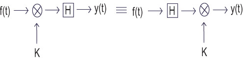
A block diagram demonstrating the scaling property of linearity
To demonstrate that a system H obeys the superposition property of linearity is to show that H(f 1(t) + f 2(t)) = H(f 1(t)) + H(f 2(t))
Figure 2.2.

A block diagram demonstrating the superposition property of linearity
It is possible to check a system for linearity in a single (though larger) step. To do this, simply combine the first two steps to get H(k 1 f 1(t) + k 2 f 2(t)) = k 2 H(f 1(t)) + k 2 H(f 2(t))
Time Invariant vs. Time Varying
A system is said to be time invariant if it commutes with the parameter shift operator defined by S T ( f ( t ) ) = f ( t – T ) for all T , which is to say
(2.1)H S T = S T H
for all real T . Intuitively, that means that for any input function that produces some output function, any time shift of that input function will produce an output function identical in every way except that it is shifted by the same amount. Any system that does not have this property is said to be time varying.
Figure 2.3.
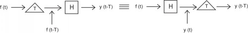
This block diagram shows what the condition for time invariance. The output is the same whether the delay is put on the input or the output.
Causal vs. Noncausal
A causal system is one in which the output depends only on current or past inputs, but not future inputs. Similarly, an anticausal system is one in which the output depends only on current or future inputs, but not past inputs. Finally, a noncausal system is one in which the output depends on both past and future inputs. All "realtime" systems must be causal, since they can not have future inputs available to them.
One may think the idea of future inputs does not seem to make much physical sense; however, we have only been dealing with time as our dependent variable so far, which is not always the case. Imagine rather that we wanted to do image processing. Then the dependent variable might represent pixel positions to the left and right (the "future") of the current position on the image, and we would not necessarily have a causal system.
Figure 2.4.
(a) For a typical system to be causal...
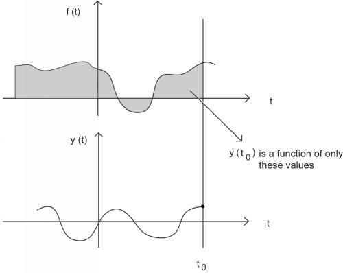
(b) ...the output at time t 0 , y(t 0) , can only depend on the portion of the input signal before t 0 .
Stable vs. Unstable
There are several definitions of stability, but the one that will be used most frequently in this course will be bounded input, bounded output (BIBO) stability. In this context, a stable system is one in which the output is bounded if the input is also bounded. Similarly, an unstable system is one in which at least one bounded input produces an unbounded output.
Representing this mathematically, a stable system must have the following property, where x(t) is the input and y(t) is the output. The output must satisfy the condition |y(t)| ≤ M y < ∞ whenever we have an input to the system that satisfies |x(t)| ≤ M x < ∞ M x and M y both represent a set of finite positive numbers and these relationships hold for all of t . Otherwise, the system is unstable.
System Classifications Summary
This module describes just some of the many ways in which systems can be classified. Systems can be continuous time, discrete time, or neither. They can be linear or nonlinear, time invariant or time varying, and stable or unstable. We can also divide them based on their causality properties. There are other ways to classify systems, such as use of memory, that are not discussed here but will be described in subsequent modules.
2.2. Linear Time Invariant Systems*
Introduction
Linearity and time invariance are two system properties that greatly simplify the study of systems that exhibit them. In our study of signals and systems, we will be especially interested in systems that demonstrate both of these properties, which together allow the use of some of the most powerful tools of signal processing.
Linear Time Invariant Systems
Linear Systems
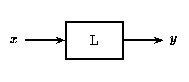
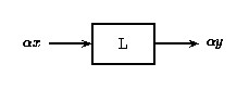
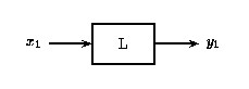
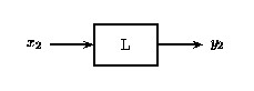
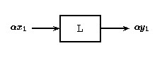
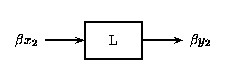
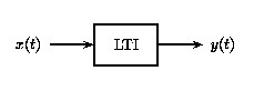
If a system is linear, this means that when an input to a given system is scaled by a value, the output of the system is scaled by the same amount.
Figure 2.5. Linear Scaling
(a)
(b)
In Figure 2.5 above, an input x to the linear system L gives the output y . If x is scaled by a value α and passed through this same system, as in Figure 2.5, the output will also be scaled by α .
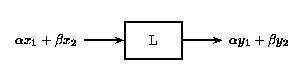
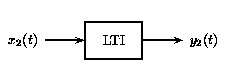
A linear system also obeys the principle of superposition. This means that if two inputs are added together and passed through a linear system, the output will be the sum of the individual inputs' outputs.
Figure 2.6.
(a)
(b)
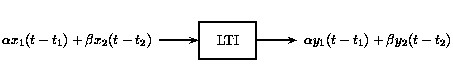
Figure 2.7. Superposition Principle
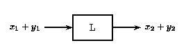
If Figure 2.6 is true, then the principle of superposition says that Figure 2.7 is true as well. This holds for linear systems.
That is, if Figure 2.6 is true, then Figure 2.7 is also true for a linear system. The scaling property mentioned above still holds in conjunction with the superposition principle. Therefore, if the inputs x and y are scaled by factors α and β, respectively, then the sum of these scaled inputs will give the sum of the individual scaled outputs:
Figure 2.8.
(a)
(b)
Figure 2.9. Superposition Principle with Linear Scaling
Given Figure 2.8 for a linear system, Figure 2.9 holds as well.
Example 2.1.
Consider the system H 1 in which
(2.2)H 1 ( f ( t ) ) = t f ( t )
for all signals f . Given any two signals f,g and scalars a,b
(2.3)H 1 ( a f ( t ) + b g ( t ) ) ) = t ( a f ( t ) + b g ( t ) ) = a t f ( t ) + b t g ( t ) = a H 1 ( f ( t ) ) + b H 1 ( g ( t ) )
for all real t . Thus, H 1 is a linear system.
Example 2.2.
Consider the system H 2 in which
(2.4)H 2 ( f ( t ) ) = ( f ( t ) ) 2
for all signals f . Because
(2.5)H 2 ( 2 t ) = 4 t 2 ≠ 2 t 2 = 2 H 2 ( t )
for nonzero t , H 2 is not a linear system.
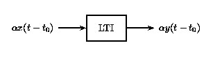
Time Invariant Systems
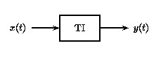
A time-invariant system has the property that a certain input will always give the same output (up to timing), without regard to when the input was applied to the system.
Figure 2.10. Time-Invariant Systems
(a)
(b)
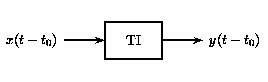
Figure 2.10 shows an input at time t while Figure 2.10 shows the same input t 0 seconds later. In a time-invariant system both outputs would be identical except that the one in Figure 2.10 would be delayed by t 0 .
In this figure, x(t) and x(t − t 0) are passed through the system TI. Because the system TI is time-invariant, the inputs x(t) and x(t − t 0) produce the same output. The only difference is that the output due to x(t − t 0) is shifted by a time t 0 .
Whether a system is time-invariant or time-varying can be seen in the differential equation (or difference equation) describing it. Time-invariant systems are modeled with constant coefficient equations. A constant coefficient differential (or difference) equation means that the parameters of the system are not changing over time and an input now will give the same result as the same input later.
Example 2.3.
Consider the system H 1 in which
(2.6)H 1 ( f ( t ) ) = t f ( t )
for all signals f . Because
(2.7)

for nonzero T , H 1 is not a time invariant system.
Example 2.4.
Consider the system H 2 in which
(2.8)H 2 ( f ( t ) ) = ( f ( t ) ) 2
for all signals f . For all real T and signals f ,
(2.9)

for all real t . Thus, H 2 is a time invariant system.
Linear Time Invariant Systems
Certain systems are both linear and time-invariant, and are thus referred to as LTI systems.
Figure 2.11. Linear Time-Invariant Systems
(a)
(b)
This is a combination of the two cases above. Since the input to Figure 2.11 is a scaled, time-shifted version of the input in Figure 2.11, so is the output.
As LTI systems are a subset of linear systems, they obey the principle of superposition. In the figure below, we see the effect of applying time-invariance to the superposition definition in the linear systems section above.
Figure 2.12.

(a)
(b)
Figure 2.13. Superposition in Linear Time-Invariant Systems
The principle of superposition applied to LTI systems
LTI Systems in Series
If two or more LTI systems are in series with each other, their order can be interchanged without affecting the overall output of the system. Systems in series are also called cascaded systems.
Figure 2.14. Cascaded LTI Systems
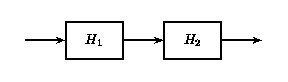
(a)
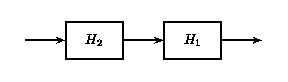
(b)
The order of cascaded LTI systems can be interchanged without changing the overall effect.
LTI Systems in Parallel
If two or more LTI systems are in parallel with one another, an equivalent system is one that is defined as the sum of these individual systems.
Figure 2.15. Parallel LTI Systems
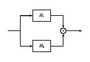
(a)
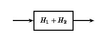
(b)
Parallel systems can be condensed into the sum of systems.
Example 2.5.
Consider the system H 3 in which
(2.10)H 3 ( f ( t ) ) = 2 f ( t )
for all signals f . Given any two signals f,g and scalars a,b
(2.11)H 3 ( a f ( t ) + b g ( t ) ) ) = 2 ( a f ( t ) + b g ( t ) ) = a 2 f ( t ) + b 2 g ( t ) = a H 3 ( f ( t ) ) + b H 3 ( g ( t ) )
for all real t . Thus, H 3 is a linear system. For all real T and signals f ,
(2.12)

for all real t . Thus, H 3 is a time invariant system. Therefore, H 3 is a linear time invariant system.
Example 2.6.
As has been previously shown, each of the following systems are not linear or not time invariant.
(2.13)H 1 ( f ( t ) ) = t f ( t )
(2.14)H 2 ( f ( t ) ) = ( f ( t ) ) 2
Thus, they are not linear time invariant systems.
Linear Time Invariant Demonstration
Figure 2.16.

Interact(when online) with the Mathematica CDF above demonstrating Linear Time Invariant systems. To download, right click and save file as .cdf.
LTI Systems Summary
Two very important and useful properties of systems have just been described in detail. The first of these, linearity, allows us the knowledge that a sum of input signals produces an output signal that is the summed original output signals and that a scaled input signal produces an output signal scaled from the original output signal. The second of these, time invariance, ensures that time shifts commute with application of the system. In other words, the output signal for a time shifted input is the same as the output signal for the original input signal, except for an identical shift in time. Systems that demonstrate both linearity and time invariance, which are given the acronym LTI systems, are particularly simple to study as these properties allow us to leverage some of the most powerful tools in signal processing.
Chapter 3. Time Domain Analysis of Continuous Time Systems
3.1. Continuous Time Systems*
Introduction
As you already now know, a continuous time system operates on a continuous time signal input and produces a continuous time signal output. There are numerous examples of useful continuous time systems in signal processing as they essentially describe the world around us. The class of continuous time systems that are both linear and time invariant, known as continuous time LTI systems, is of particular interest as the properties of linearity and time invariance together allow the use of some of the most important and powerful tools in signal processing.
Continuous Time Systems
Linearity and Time Invariance
A system H is said to be linear if it satisfies two important conditions. The first, additivity, states for every pair of signals x,y that H(x + y) = H(x) + H(y). The second, homogeneity of degree one, states for every signal x and scalar a we have H(a x) = a H(x). It is clear that these conditions can be combined together into a single condition for linearity. Thus, a system is said to be linear if for every signals x,y and scalars a,b we have that
(3.1)H ( a x + b y ) = a H ( x ) + b H ( y ) .
Linearity is a particularly important property of systems as it allows us to leverage the powerful tools of linear algebra, such as bases, eigenvectors, and eigenvalues, in their study.
A system H is said to be time invariant if a time shift of an input produces the corresponding shifted output. In other, more precise words, the system H commutes with the time shift operator S T for every T ∈ R. That is,
(3.2)S T H = H S T .
Time invariance is desirable because it eases computation while mirroring our intuition that, all else equal, physical systems should react the same to identical inputs at different times.
When a system exhibits both of these important properties it allows for a more straigtforward analysis than would otherwise be possible. As will be explained and proven in subsequent modules, computation of the system output for a given input becomes a simple matter of convolving the input with the system's impulse response signal. Also proven later, the fact that complex exponential are eigenvectors of linear time invariant systems will enable the use of frequency domain tools such as the various Fouier transforms and associated transfer functions, to describe the behavior of linear time invariant systems.
Example 3.1.
Consider the system H in which
(3.3)H ( f ( t ) ) = 2 f ( t )
for all signals f . Given any two signals f,g and scalars a,b
(3.4)H ( a f ( t ) + b g ( t ) ) ) = 2 ( a f ( t ) + b g ( t ) ) = a 2 f ( t ) + b 2 g ( t ) = a H ( f ( t ) ) + b H ( g ( t ) )
for all real t . Thus, H is a linear system. For all real T and signals f ,
(3.5)

for all real t . Thus, H is a time invariant system. Therefore, H is a linear time invariant system.
Differential Equation Representation
It is often useful to to describe systems using equations involving the rate of change in some quantity. For continuous time systems, such equations are called differential equations. One important class of differential equations is the set of linear constant coefficient ordinary differential equations, which are described in more detail in subsequent modules.
Example 3.2.
Consider the series RLC circuit shown in Figure 3.1. This system can be modeled using differential equations. We can use the voltage equations for each circuit element and Kirchoff's voltage law to write a second order linear constant coefficient differential equation describing the charge on the capacitor.
The voltage across the battery is simply V . The voltage across the capacitor is. The voltage across the resistor is
. Finally, the voltage across the inductor is
. Therefore, by Kirchoff's voltage law, it follows that
(3.6)

Figure 3.1.
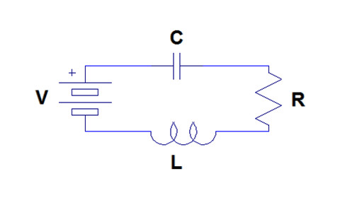
A series RLC circuit.
Continuous Time Systems Summary
Many useful continuous time systems will be encountered in a study of signals and systems. This course is most interested in those that demonstrate both the linearity property and the time invariance property, which together enable the use of some of the most powerful tools of signal processing. It is often useful to describe them in terms of rates of change through linear constant coefficient ordinary differential equations.
3.2. Continuous Time Impulse Response*
Introduction
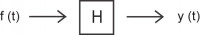
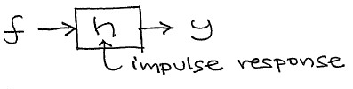
| The output of an LTI system is completely determined by the input and the system's response to a unit impulse.
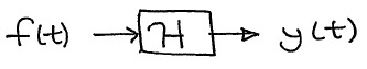
Figure 3.2. System Output
We can determine the system's output, y(t), if we know the system's impulse response, h(t), and the input, f(t). |
| The output for a unit impulse input is called the impulse response.
Figure 3.3.
|
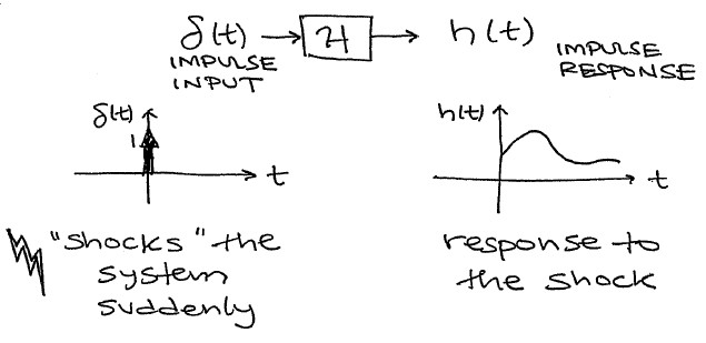
Example Approximate Impulses
Hammer blow to a structure
Hand clap or gun blast in a room
Air gun blast underwater
LTI Systems and Impulse Responses
Finding System Outputs
By the sifting property of impulses, any signal can be decomposed in terms of an integral of shifted, scaled impulses.
(3.7)
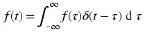
δ(t − τ) peaks up where t = τ .
Figure 3.4.
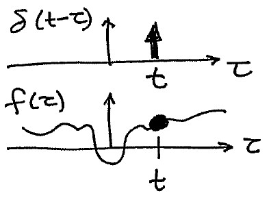
Since we know the response of the system to an impulse and any signal can be decomposed into impulses, all we need to do to find the response of the system to any signal is to decompose the signal into impulses, calculate the system's output for every impulse and add the outputs back together. This is the process known as Convolution. Since we are in Continuous Time, this is the Continuous Time Convolution Integral.
Finding Impulse Responses
| Theory:
| |
| Practice:
| |
We will assume that h(t) is given for now.
|
Impulse Response Summary
When a system is "shocked" by a delta function, it produces an output known as its impulse response. For an LTI system, the impulse response completely determines the output of the system given any arbitrary input. The output can be found using continuous time convolution.
3.3. Continuous Time Convolution*
Introduction
Convolution, one of the most important concepts in electrical engineering, can be used to determine the output a system produces for a given input signal. It can be shown that a linear time invariant system is completely characterized by its impulse response. The sifting property of the continuous time impulse function tells us that the input signal to a system can be represented as an integral of scaled and shifted impulses and, therefore, as the limit of a sum of scaled and shifted approximate unit impulses. Thus, by linearity, it would seem reasonable to compute of the output signal as the limit of a sum of scaled and shifted unit impulse responses and, therefore, as the integral of a scaled and shifted impulse response. That is exactly what the operation of convolution accomplishes. Hence, convolution can be used to determine a linear time invariant system's output from knowledge of the input and the impulse response.
Convolution and Circular Convolution
Convolution
Operation Definition
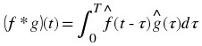
Continuous time convolution is an operation on two continuous time signals defined by the integral
(3.8) ( f * g ) ( t ) = ∫∞ – ∞ f ( τ ) g ( t – τ ) d τ
for all signals f,g defined on R. It is important to note that the operation of convolution is commutative, meaning that
(3.9)f * g = g * f
for all signals f,g defined on R. Thus, the convolution operation could have been just as easily stated using the equivalent definition
(3.10) ( f * g ) ( t ) = ∫∞ – ∞ f ( t – τ ) g ( τ ) d τ
for all signals f,g defined on R. Convolution has several other important properties not listed here but explained and derived in a later module.
Definition Motivation
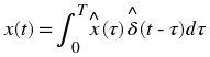
The above operation definition has been chosen to be particularly useful in the study of linear time invariant systems. In order to see this, consider a linear time invariant system H with unit impulse response h . Given a system input signal x we would like to compute the system output signal H(x). First, we note that the input can be expressed as the convolution
(3.11)x ( t ) = ∫∞ – ∞ x ( τ ) δ ( t – τ ) d τ
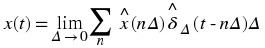
by the sifting property of the unit impulse function. Writing this integral as the limit of a summation,
(3.12)

where
(3.13)
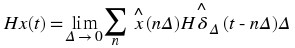
approximates the properties of δ(t). By linearity
(3.14)
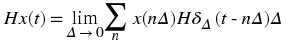
which evaluated as an integral gives
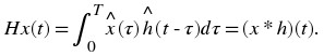
(3.15)H x ( t ) = ∫∞ – ∞ x ( τ ) H δ ( t – τ ) d τ .
Since H δ(t – τ) is the shifted unit impulse response h(t – τ), this gives the result
(3.16)H x ( t ) = ∫∞ – ∞ x ( τ ) h ( t – τ ) d τ = ( x * h ) ( t ) .
Hence, convolution has been defined such that the output of a linear time invariant system is given by the convolution of the system input with the system unit impulse response.
Graphical Intuition
It is often helpful to be able to visualize the computation of a convolution in terms of graphical processes. Consider the convolution of two functions f,g given by
(3.17) ( f * g ) ( t ) = ∫∞ – ∞ f ( τ ) g ( t – τ ) d τ = ∫∞ – ∞ f ( t – τ ) g ( τ ) d τ .
The first step in graphically understanding the operation of convolution is to plot each of the functions. Next, one of the functions must be selected, and its plot reflected across the τ = 0 axis. For each real t , that same function must be shifted left by t . The product of the two resulting plots is then constructed. Finally, the area under the resulting curve is computed.
Example 3.3.
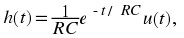
Recall that the impulse response for the capacitor voltage in a series RC circuit is given by
(3.18)
and consider the response to the input voltage
(3.19)x ( t ) = u ( t ) .
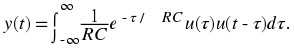
We know that the output for this input voltage is given by the convolution of the impulse response with the input signal
(3.20)y ( t ) = x ( t ) * h ( t ) .
We would like to compute this operation by beginning in a way that minimizes the algebraic complexity of the expression. Thus, since x(t) = u(t) is the simpler of the two signals, it is desirable to select it for time reversal and shifting. Thus, we would like to compute
(3.21)
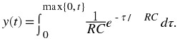
The step functions can be used to further simplify this integral by narrowing the region of integration to the nonzero region of the integrand. Therefore,
(3.22)
Hence, the output is
(3.23)
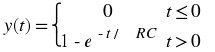
which can also be written as
(3.24)y ( t ) = (1 – e – t / R C ) u ( t ) .
Circular Convolution
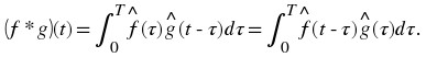
Continuous time circular convolution is an operation on two finite length or periodic continuous time signals defined by the integral
(3.25)

for all signals f,g defined on R[0,T] where  are periodic extensions of f and g . It is important to note that the operation of circular convolution is commutative, meaning that
(3.26)f * g = g * f
for all signals f,g defined on R[0,T]. Thus, the circular convolution operation could have been just as easily stated using the equivalent definition
(3.27)
for all signals f,g defined on R[0,T] where  are periodic extensions of f and g . Circular convolution has several other important properties not listed here but explained and derived in a later module.
Alternatively, continuous time circular convolution can be expressed as the sum of two integrals given by
(3.28) ( f * g ) ( t ) = ∫0 t f ( τ ) g ( t – τ ) d τ + ∫t T f ( τ ) g ( t – τ + T ) d τ
for all signals f,g defined on R[0,T].
Meaningful examples of computing continuous time circular convolutions in the time domain would involve complicated algebraic manipulations dealing with the wrap around behavior, which would ultimately be more confusing than helpful. Thus, none will be provided in this section. However, continuous time circular convolutions are more easily computed using frequency domain tools as will be shown in the continuous time Fourier series section.
Definition Motivation
The above operation definition has been chosen to be particularly useful in the study of linear time invariant systems. In order to see this, consider a linear time invariant system H with unit impulse response h . Given a finite or periodic system input signal x we would like to compute the system output signal H(x). First, we note that the input can be expressed as the circular convolution
(3.29)
by the sifting property of the unit impulse function. Writing this integral as the limit of a summation,
(3.30)
where
(3.31)

approximates the properties of δ(t). By linearity
(3.32)
which evaluated as an integral gives
(3.33)

Since H δ(t – τ) is the shifted unit impulse response h(t – τ), this gives the result
(3.34)
Hence, circular convolution has been defined such that the output of a linear time invariant system is given by the convolution of the system input with the system unit impulse response.
Graphical Intuition
It is often helpful to be able to visualize the computation of a circular convolution in terms of graphical processes. Consider the circular convolution of two finite length functions f,g given by
(3.35)
The first step in graphically understanding the operation of convolution is to plot each of the periodic extensions of the functions. Next, one of the functions must be selected, and its plot reflected across the τ = 0 axis. For each t ∈ R[0,T], that same function must be shifted left by t . The product of the two resulting plots is then constructed. Finally, the area under the resulting curve on R[0,T] is computed.
Convolution Demonstration
Figure 3.6.
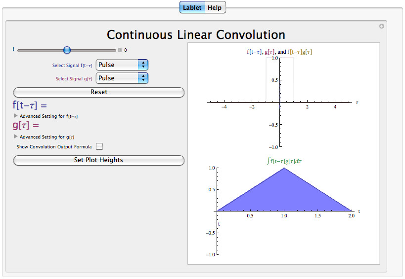
Interact (when online) with a Mathematica CDF demonstrating Convolution. To Download, right-click and save target as .cdf.
Convolution Summary
Convolution, one of the most important concepts in electrical engineering, can be used to determine the output signal of a linear time invariant system for a given input signal with knowledge of the system's unit impulse response. The operation of continuous time convolution is defined such that it performs this function for infinite length continuous time signals and systems. The operation of continuous time circular convolution is defined such that it performs this function for finite length and periodic continuous time signals. In each case, the output of the system is the convolution or circular convolution of the input signal with the unit impulse response.
3.4. Properties of Continuous Time Convolution*
Introduction
We have already shown the important role that continuous time convolution plays in signal processing. This section provides discussion and proof of some of the important properties of continuous time convolution. Analogous properties can be shown for continuous time circular convolution with trivial modification of the proofs provided except where explicitly noted otherwise.
Continuous Time Convolution Properties
Associativity
The operation of convolution is associative. That is, for all continuous time signals f 1,f 2,f 3 the following relationship holds.
(3.36)

In order to show this, note that
(3.37)
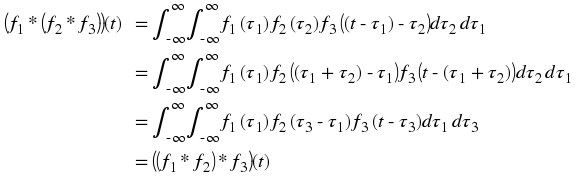
proving the relationship as desired through the substitution τ 3 = τ 1 + τ 2 .
Commutativity
The operation of convolution is commutative. That is, for all continuous time signals f 1,f 2 the following relationship holds.
(3.38)f 1 * f 2 = f 2 * f 1
In order to show this, note that
(3.39)
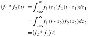
proving the relationship as desired through the substitution τ 2 = t – τ 1 .
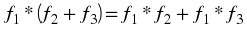
Distribitivity
The operation of convolution is distributive over the operation of addition. That is, for all continuous time signals f 1,f 2,f 3 the following relationship holds.
(3.40)
In order to show this, note that
(3.41)
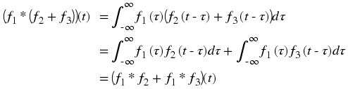
proving the relationship as desired.
Multilinearity
The operation of convolution is linear in each of the two function variables. Additivity in each variable results from distributivity of convolution over addition. Homogenity of order one in each varible results from the fact that for all continuous time signals f 1,f 2 and scalars a the following relationship holds.
(3.42)

In order to show this, note that
(3.43)
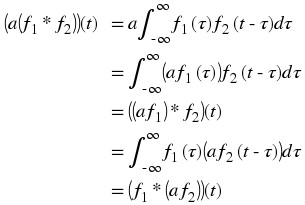
proving the relationship as desired.
Conjugation
The operation of convolution has the following property for all continuous time signals f 1,f 2 .
(3.44)

In order to show this, note that
(3.45)
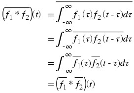
proving the relationship as desired.
Time Shift
The operation of convolution has the following property for all continuous time signals f 1,f 2 where S T is the time shift operator.
(3.46)

In order to show this, note that
(3.47)
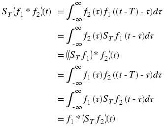
proving the relationship as desired.
Differentiation
The operation of convolution has the following property for all continuous time signals f 1,f 2 .
(3.48)
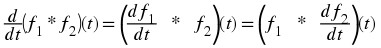
In order to show this, note that
(3.49)
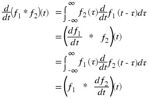
proving the relationship as desired.
Impulse Convolution
The operation of convolution has the following property for all continuous time signals f where δ is the Dirac delta funciton.
(3.50)f * δ = f
In order to show this, note that
(3.51)
proving the relationship as desired.
Width
The operation of convolution has the following property for all continuous time signals f 1,f 2 where Duration(f) gives the duration of a signal f .
(3.52)

. In order to show this informally, note that  is nonzero for all t for which there is a τ such that f
1(τ)f
2(t – τ) is nonzero. When viewing one function as reversed and sliding past the other, it is easy to see that such a τ exists for all t on an interval of length
is nonzero for all t for which there is a τ such that f
1(τ)f
2(t – τ) is nonzero. When viewing one function as reversed and sliding past the other, it is easy to see that such a τ exists for all t on an interval of length  . Note that this is not always true of circular convolution of finite length and periodic signals as there is then a maximum possible duration within a period.
Convolution Properties Summary
As can be seen the operation of continuous time convolution has several important properties that have been listed and proven in this module. With slight modifications to proofs, most of these also extend to continuous time circular convolution as well and the cases in which exceptions occur have been noted above. These identities will be useful to keep in mind as the reader continues to study signals and systems.
3.5. Eigenfunctions of Continuous Time LTI Systems*
Introduction
Prior to reading this module, the reader should already have some experience with linear algebra and should specifically be familiar with the eigenvectors and eigenvalues of linear operators. A linear time invariant system is a linear operator defined on a function space that commutes with every time shift operator on that function space. Thus, we can also consider the eigenvector functions, or eigenfunctions, of a system. It is particularly easy to calculate the output of a system when an eigenfunction is the input as the output is simply the eigenfunction scaled by the associated eigenvalue. As will be shown, continuous time complex exponentials serve as eigenfunctions of linear time invariant systems operating on continuous time signals.
Eigenfunctions of LTI Systems
Consider a linear time invariant system H with impulse response h operating on some space of infinite length continuous time signals. Recall that the output H(x(t)) of the system for a given input x(t) is given by the continuous time convolution of the impulse response with the input
(3.53)H ( x ( t ) ) = ∫∞ – ∞ h ( τ ) x ( t – τ ) d τ .
Now consider the input x(t) = e st where s ∈ C. Computing the output for this input,
(3.54)
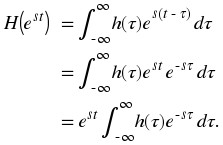
Thus,
(3.55)
where
(3.56)λ s = ∫∞ – ∞ h ( τ ) e – s τ d τ
is the eigenvalue corresponding to the eigenvector e st .
There are some additional points that should be mentioned. Note that, there still may be additional eigenvalues of a linear time invariant system not described by e st for some s ∈ C. Furthermore, the above discussion has been somewhat formally loose as e st may or may not belong to the space on which the system operates. However, for our purposes, complex exponentials will be accepted as eigenvectors of linear time invariant systems. A similar argument using continuous time circular convolution would also hold for spaces finite length signals.
Eigenfunction of LTI Systems Summary
As has been shown, continuous time complex exponential are eigenfunctions of linear time invariant systems operating on continuous time signals. Thus, it is particularly simple to calculate the output of a linear time invariant system for a complex exponential input as the result is a complex exponential output scaled by the associated eigenvalue. Consequently, representations of continuous time signals in terms of continuous time complex exponentials provide an advantage when studying signals. As will be explained later, this is what is accomplished by the continuous time Fourier transform and continuous time Fourier series, which apply to aperiodic and periodic signals respectively.
3.6. BIBO Stability of Continuous Time Systems*
Introduction
BIBO stability stands for bounded input, bounded output stability. BIBO stablity is the system property that any bounded input yields a bounded output. This is to say that as long as we input a signal with absolute value less than some constant, we are guaranteed to have an output with absolute value less than some other constant.
Continuous Time BIBO Stability
In order to understand this concept, we must first look more closely into exactly what we mean by bounded. A bounded signal is any signal such that there exists a value such that the absolute value of the signal is never greater than some value. Since this value is arbitrary, what we mean is that at no point can the signal tend to infinity, including the end behavior.
Figure 3.7.
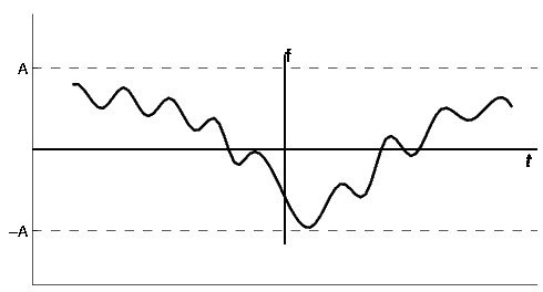
A bounded signal is a signal for which there exists a constant A such that |f(t)| < A
Time Domain Conditions
Now that we have identified what it means for a signal to be bounded, we must turn our attention to the condition a system must possess in order to guarantee that if any bounded signal is passed through the system, a bounded signal will arise on the output. It turns out that a continuous time LTI system with impulse response h(t) is BIBO stable if and only if
(3.57)
Continuous-Time Condition for BIBO Stability
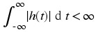
This is to say that the impulse response is absolutely integrable.
Laplace Domain Conditions
Stability is very easy to infer from the pole-zero plot of a transfer function. The only condition necessary to demonstrate stability is to show that the ⅈω -axis is in the region of convergence. Consequently, for stable causal systems, all poles must be to the left of the imaginary axis.
Figure 3.8.
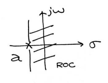
(a) Example of a pole-zero plot for a stable continuous-time system.
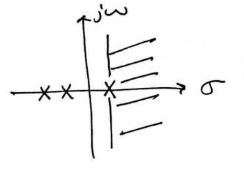
(b) Example of a pole-zero plot for an unstable continuous-time system.
BIBO Stability Summary
Bounded input bounded output stability, also known as BIBO stability, is an important and generally desirable system characteristic. A system is BIBO stable if every bounded input signal results in a bounded output signal, where boundedness is the property that the absolute value of a signal does not exceed some finite constant. In terms of time domain features, a continuous time system is BIBO stable if and only if its impulse response is absolutely integrable. Equivalently, in terms of Laplace domain features, a continuous time system is BIBO stable if and only if the region of convergence of the transfer function includes the imaginary axis.
3.7. Linear Constant Coefficient Differential Equations*
Introduction: Ordinary Differential Equations
In our study of signals and systems, it will often be useful to describe systems using equations involving the rate of change in some quantity. Such equations are called differential equations. For instance, you may remember from a past physics course that an object experiences simple harmonic motion when it has an acceleration that is proportional to the magnitude of its displacement and opposite in direction. Thus, this system is described as the differential equation shown in Equation 3.58.
(3.58)

Because the differential equation in Equation 3.58 has only one independent variable and only has derivatives with respect to that variable, it is called an ordinary differential equation. There are more complicated differential equations, such as the Schrodinger equation, which involve derivatives with respect to multiple independent variables. These are called partial differential equations, but they are not within the scope of this module.
Given a sufficiently descriptive set of initial conditions or boundary conditions, if there is a solution to the differential equation, that solution is unique and describes the behavior of the system. Of course, the results are only accurate to the degree that the model mirrors reality.
Linear Constant Coefficient Ordinary Differential Equations
An important subclass of ordinary differential equations is the set of linear constant coefficient ordinary differential equations. These equations are of the form
(3.59)A x ( t ) = f ( t )
where A is a differential operator of the form given in Equation 3.60.
(3.60)
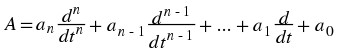
Note that operators of this type satisfy the linearity conditions, and a 1,...,a n are real constants. Furthermore, Equation Equation 3.59 with these operators has derivatives with respect to only one variable, making it an ordinary differential equation.
A similar concept for a discrete time setting, difference equations, is discussed in the chapter on time domain analysis of discrete time systems. There are many parallels between the discussion of linear constant coefficient ordinary differential equations and linear constant coefficient differece equations.
Applications of Differential Equations
Consider the decay model in which a quantity of an unstable isotope decreases at a rate proportional to the quanity of unstable isotope remaining. Thus, the decay of the isotope is modeled by the first order linear constant coefficient differential equation
(3.61)

where r is some real rate.
Now consider the series RLC circuit shown in Figure 3.9. This system can be modeled using differential equations. We can use the voltage equations for each circuit element and Kirchoff's voltage law to write a second order linear constant coefficient differential equation describing the charge on the capacitor.
The voltage across the battery is simply V . The voltage across the capacitor is  . The voltage across the resistor is
  . Finally, the voltage across the inductor is
  . Therefore, by Kirchoff's voltage law, it follows that
(3.62)

Figure 3.9.

A series RLC circuit.
The section Solving Linear Constant Coefficient Differential Equations will describe in depth how solutions to differential equations like those in the examples may be obtained.
Linear Constant Coefficient Oridinary Differential Equations Summary
Differential equations are an important mathematical tool for modeling continuous time systems. An important subclass of these is the class of linear constant coefficient ordinary differential equations. Linear constant coefficient ordinary differential equations are often particularly easy to solve as will be described in the module on solutions to linear constant coefficient ordinary differential equations and are useful in describing a wide range of situations that arise in electrical engineering and in other fields.
3.8. Solving Linear Constant Coefficient Differential Equations*
Introduction
The approach to solving linear constant coefficient ordinary differential equations is to find the general form of all possible solutions to the equation and then apply a number of conditions to find the appropriate solution. The two main types of problems are initial value problems, which involve constraints on the solution and its derivatives at a single point, and boundary value problems, which involve constraints on the solution or its derivatives at several points.
The number of initial conditions needed for an N th order differential equation, which is the order of the highest order derivative, is N , and a unique solution is always guaranteed if these are supplied. Boundary value problems can be slightly more complicated and will not necessarily have a unique solution or even a solution at all for a given set of conditions. Thus, this module will focus exclusively on initial value problems.
Solving Linear Constant Coefficient Ordinary Differential Equations
Consider some linear constant coefficient ordinary differential equation given by A x(t) = f(t), where A is a differential operator of the form
(3.63)

Let x
h
(t) and x
p
(t) be two functions such that A
x
h
(t) = 0 and A
x
p
(t) = f(t). By the linearity of A , note that  . Thus, the form of the general solution x
g
(t) to any linear constant coefficient ordinary differential equation is the sum of a homogeneous solution x
h
(t) to the equation A
x = 0 and a particular solution x
p
(t) that is specific to the forcing function f(t).
. Thus, the form of the general solution x
g
(t) to any linear constant coefficient ordinary differential equation is the sum of a homogeneous solution x
h
(t) to the equation A
x = 0 and a particular solution x
p
(t) that is specific to the forcing function f(t).
We wish to determine the forms of the homogeneous and nonhomogeneous solutions in full generality in order to avoid incorrectly restricting the form of the solution before applying any conditions. Otherwise, a valid set of initial or boundary conditions might appear to have no corresponding solution trajectory. The following discussion shows how to accomplish this for linear constant coefficient ordinary differential equations.
Finding the Homogeneous Solution
In order to find the homogeneous solution to A x(t) = f(t), consider the differential equation A x(t) = 0. We know that the solutions have the form c e λt for some complex constants c,λ . Since A c e λt = 0 for a solution, it follows that
(3.64)

so it also follows that
(3.65)a n λ n + a n – 1 λ n – 1 . . . + a 1 λ + a 0 = 0 .
Therefore, the parameters of the solution exponents are the roots of the above polynomial, called the characteristic polynomial.
For equations of order two or more, there will be several roots. If all of the roots are distinct, then the the general form of the homogeneous solution is simply
(3.66)x h ( t ) = c 1 e λ 1 t + . . . + c n e λ n t .
If a root has multiplicity that is greater than one, the repeated solutions must be multiplied by each powers of t from 0 to one less than the root multiplicity (in order to ensure linearly independent solutions). For instance, if λ 1 had multiplicity 2 and λ 2 had multiplicity 3, the homogeneous solution would be
(3.67)x h ( t ) = c 1 e λ 1 t + c 2 t e λ 1 t + c 3 e λ 2 t + c 4 t e λ 2 t + c 5 t 2 e λ 2 t .
Example 3.4.
Consider the decay model in which a quantity of an unstable isotope decreases at a rate proportional to the quanity of unstable isotope remaining. Thus, the decay of the isotope is modeled by the first order linear constant coefficient differential equation
(3.68)

where r is some real rate. This differential equation could easily be solved through straightforward integration. However, the methods described above will be used instead. Note that the forcing function is zero, so only a homogenous solution is needed. It is easy to see that the characteristic polynomial is λ + r = 0, so there is one root λ 1 = r . Thus the solution is of the form
(3.69)x ( t ) = c 1 e rt .
Given a rate and an initial condition, this can be applied to a specific situation. For instance, we know that carbon-14 decays at a rate of approximately r = 1.21x10 – 4 year – 1 , and if we normalize the natural concentration of carbon-14 to x(0) = 1 the solution becomes x(t) = e – 1.21x10 – 4 t . Knowledge of this curve would be useful for radioisotope based dating.
Finding the Particular Solution
Finding the particular solution is slightly more complicated task than finding the homogeneous solution. A formal method, called variation of parameters accomplishes this, and there are also several heuristics that can be used. It can also be found through convolution of the input with the unit impulse response, once the unit impulse response is known. Finding the particular solution to a differential equation is discussed further in the chapter concerning the Laplace transform, which greatly simplifies the procedure for solving linear constant coefficient ordinary differential equations using frequency domain tools.
Example 3.5.
Consider the series RLC circuit shown in Figure 3.10. This system can be modeled using differential equations. We can use the voltage equations for each circuit element and Kirchoff's voltage law to write a second order linear constant coefficient differential equation describing the charge on the capacitor.
The voltage across the battery is simply V . The voltage across the capacitor is. The voltage across the resistor is
. Finally, the voltage across the inductor is
. Therefore, by Kirchoff's voltage law, it follows that
(3.70)
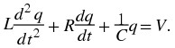
Figure 3.10.

A series RLC circuit.
First, the homogeneous solution is found. It is easy to see that the characteristic polynomial is. Therefore, the two roots are
and
. Often, these are stated in terms of the attenuation factor
and the resonant frequency
. Thus,
and
.
Thus, the homogeneous equation is of the form
(3.71)
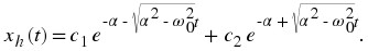
It turns out that the response to the constant voltage source forcing function is a constant, so
(3.72)x p ( t ) = V C .
Hence, the general solution is
(3.73)
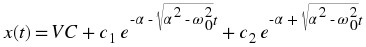
where c 1 and c 2 depend on the initial conditions. The system demonstrates a rich array of behaviors based on the relative values of α and ω 0 , which the reader is encouraged to explore.
Solving Differential Equations Summary
Linear constant coefficient ordinary differential equations are useful for modeling a wide variety of continuous time systems. The approach to solving them is to find the general form of all possible solutions to the equation and then apply a number of conditions to find the appropriate solution. This is done by finding the homogeneous solution to the differential equation that does not depend on the forcing function input and a particular solution to the differential equation that does depend on the forcing function input.
Chapter 4. Time Domain Analysis of Discrete Time Systems
4.1. Discrete Time Systems*
Introduction
As you already now know, a discrete time system operates on a discrete time signal input and produces a discrete time signal output. There are numerous examples of useful discrete time systems in digital signal processing, such as digital filters for images or sound. The class of discrete time systems that are both linear and time invariant, known as discrete time LTI systems, is of particular interest as the properties of linearity and time invariance together allow the use of some of the most important and powerful tools in signal processing.
Discrete Time Systems
Linearity and Time Invariance
A system H is said to be linear if it satisfies two important conditions. The first, additivity, states for every pair of signals x,y that H(x + y) = H(x) + H(y). The second, homogeneity of degree one, states for every signal x and scalar a we have H(a x) = a H(x). It is clear that these conditions can be combined together into a single condition for linearity. Thus, a system is said to be linear if for every signals x,y and scalars a,b we have that
(4.1)H ( a x + b y ) = a H ( x ) + b H ( y ) .
Linearity is a particularly important property of systems as it allows us to leverage the powerful tools of linear algebra, such as bases, eigenvectors, and eigenvalues, in their study.
A system H is said to be time invariant if a time shift of an input produces the corresponding shifted output. In other, more precise words, the system H commutes with the time shift operator S T for every T ∈ Z. That is,
(4.2)S T H = H S T .
Time invariance is desirable because it eases computation while mirroring our intuition that, all else equal, physical systems should react the same to identical inputs at different times.
When a system exhibits both of these important properties it opens. As will be explained and proven in subsequent modules, computation of the system output for a given input becomes a simple matter of convolving the input with the system's impulse response signal. Also proven later, the fact that complex exponential are eigenvectors of linear time invariant systems will encourage the use of frequency domain tools such as the various Fouier transforms and associated transfer functions, to describe the behavior of linear time invariant systems.
Example 4.1.
Consider the system H in which
(4.3)H ( f ( n ) ) = 2 f ( n )
for all signals f . Given any two signals f,g and scalars a,b
(4.4)H ( a f ( n ) + b g ( n ) ) ) = 2 ( a f ( n ) + b g ( n ) ) = a 2 f ( n ) + b 2 g ( n ) = a H ( f ( n ) ) + b H ( g ( n ) )
for all integers n . Thus, H is a linear system. For all integers T and signals f ,
(4.5)

for all integers n . Thus, H is a time invariant system. Therefore, H is a linear time invariant system.
Difference Equation Representation
It is often useful to to describe systems using equations involving the rate of change in some quantity. For discrete time systems, such equations are called difference equations, a type of recurrence relation. One important class of difference equations is the set of linear constant coefficient difference equations, which are described in more detail in subsequent modules.
Example 4.2.
Recall that the Fibonacci sequence describes a (very unrealistic) model of what happens when a pair rabbits get left alone in a black box... The assumptions are that a pair of rabits never die and produce a pair of offspring every month starting on their second month of life. This system is defined by the recursion relation for the number of rabit pairs y(n) at month n
(4.6)y ( n ) = y ( n – 1 ) + y ( n – 2 )
with the initial conditions y(0) = 0 and y(1) = 1. The result is a very fast growth in the sequence. This is why we never leave black boxes open.
Discrete Time Systems Summary
Many useful discrete time systems will be encountered in a study of signals and systems. This course is most interested in those that demonstrate both the linearity property and the time invariance property, which together enable the use of some of the most powerful tools of signal processing. It is often useful to describe them in terms of rates of change through linear constant coefficient difference equations, a type of recurrence relation.
4.2. Discrete Time Impulse Response*
Introduction
| The output of a discrete time LTI system is completely determined by the input and the system's response to a unit impulse.
Figure 4.1. System Output
We can determine the system's output, y[n], if we know the system's impulse response, h[n], and the input, x[n]. |
| The output for a unit impulse input is called the impulse response.
Figure 4.2.
Figure 4.3.
(a)
(b) |
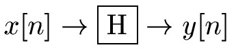

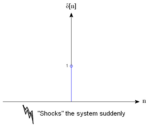
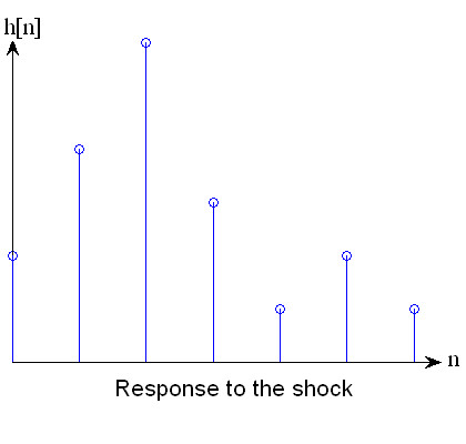
Example Impulses
Since we are considering discrete time signals and systems, an ideal impulse is easy to simulate on a computer or some other digital device. It is simply a signal that is 1 at the point n = 0, and 0 everywhere else.
LTI Systems and Impulse Responses
Finding System Outputs
By the sifting property of impulses, any signal can be decomposed in terms of an infinite sum of shifted, scaled impulses.
(4.7)
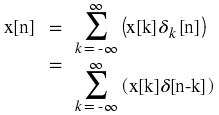
The function δ k [n] = δ[n-k] peaks up where n = k .
Figure 4.4.
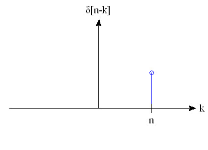
(a)
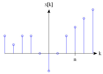
(b)
Since we know the response of the system to an impulse and any signal can be decomposed into impulses, all we need to do to find the response of the system to any signal is to decompose the signal into impulses, calculate the system's output for every impulse and add the outputs back together. This is the process known as Convolution. Since we are in Discrete Time, this is the Discrete Time Convolution Sum.
Finding Impulse Responses
| Theory:
| |
| Practice:
| |
We will assume that h[n] is given for now.
|
Impulse Response Summary
When a system is "shocked" by a delta function, it produces an output known as its impulse response. For an LTI system, the impulse response completely determines the output of the system given any arbitrary input. The output can be found using discrete time convolution.
4.3. Discrete Time Convolution*
Introduction
Convolution, one of the most important concepts in electrical engineering, can be used to determine the output a system produces for a given input signal. It can be shown that a linear time invariant system is completely characterized by its impulse response. The sifting property of the discrete time impulse function tells us that the input signal to a system can be represented as a sum of scaled and shifted unit impulses. Thus, by linearity, it would seem reasonable to compute of the output signal as the sum of scaled and shifted unit impulse responses. That is exactly what the operation of convolution accomplishes. Hence, convolution can be used to determine a linear time invariant system's output from knowledge of the input and the impulse response.
Convolution and Circular Convolution
Convolution
Operation Definition
Discrete time convolution is an operation on two discrete time signals defined by the integral
(4.8)
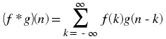
for all signals f,g defined on Z. It is important to note that the operation of convolution is commutative, meaning that
(4.9)f * g = g * f
for all signals f,g defined on Z. Thus, the convolution operation could have been just as easily stated using the equivalent definition
(4.10)
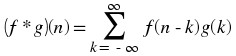
for all signals f,g defined on Z. Convolution has several other important properties not listed here but explained and derived in a later module.
Definition Motivation
The above operation definition has been chosen to be particularly useful in the study of linear time invariant systems. In order to see this, consider a linear time invariant system H with unit impulse response h . Given a system input signal x we would like to compute the system output signal H(x). First, we note that the input can be expressed as the convolution
(4.11)
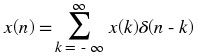
by the sifting property of the unit impulse function. By linearity
(4.12)
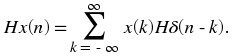
Since H δ(n – k) is the shifted unit impulse response h(n – k), this gives the result
(4.13)
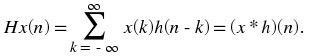
Hence, convolution has been defined such that the output of a linear time invariant system is given by the convolution of the system input with the system unit impulse response.
Graphical Intuition
It is often helpful to be able to visualize the computation of a convolution in terms of graphical processes. Consider the convolution of two functions f,g given by
(4.14)
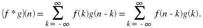
The first step in graphically understanding the operation of convolution is to plot each of the functions. Next, one of the functions must be selected, and its plot reflected across the k = 0 axis. For each real t , that same function must be shifted left by t . The product of the two resulting plots is then constructed. Finally, the area under the resulting curve is computed.
Example 4.3.
Recall that the impulse response for a discrete time echoing feedback system with gain a is
(4.15)h ( n ) = a n u ( n ) ,
and consider the response to an input signal that is another exponential
(4.16)x ( n ) = b n u ( n ) .
We know that the output for this input is given by the convolution of the impulse response with the input signal
(4.17)y ( n ) = x ( n ) * h ( n ) .
We would like to compute this operation by beginning in a way that minimizes the algebraic complexity of the expression. However, in this case, each possible coice is equally simple. Thus, we would like to compute
(4.18)
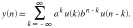
The step functions can be used to further simplify this sum. Therefore,
(4.19)y ( n ) = 0
for n < 0 and
(4.20)
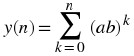
for n ≥ 0. Hence, provided a b ≠ 1, we have that
(4.21)
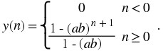
Circular Convolution
Discrete time circular convolution is an operation on two finite length or periodic discrete time signals defined by the integral
(4.22)

for all signals f,g defined on Z[0,N – 1] where  are periodic extensions of f and g . It is important to note that the operation of circular convolution is commutative, meaning that
(4.23)f * g = g * f
for all signals f,g defined on Z[0,N – 1]. Thus, the circular convolution operation could have been just as easily stated using the equivalent definition
(4.24)

for all signals f,g defined on Z[0,N – 1] where  are periodic extensions of f and g . Circular convolution has several other important properties not listed here but explained and derived in a later module.
Alternatively, discrete time circular convolution can be expressed as the sum of two summations given by
(4.25)
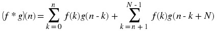
for all signals f,g defined on Z[0,N – 1].
Meaningful examples of computing discrete time circular convolutions in the time domain would involve complicated algebraic manipulations dealing with the wrap around behavior, which would ultimately be more confusing than helpful. Thus, none will be provided in this section. Of course, example computations in the time domain are easy to program and demonstrate. However, disrete time circular convolutions are more easily computed using frequency domain tools as will be shown in the discrete time Fourier series section.
Definition Motivation
The above operation definition has been chosen to be particularly useful in the study of linear time invariant systems. In order to see this, consider a linear time invariant system H with unit impulse response h . Given a finite or periodic system input signal x we would like to compute the system output signal H(x). First, we note that the input can be expressed as the circular convolution
(4.26)
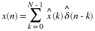
by the sifting property of the unit impulse function. By linearity,
(4.27)
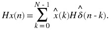
Since H δ(n – k) is the shifted unit impulse response h(n – k), this gives the result
(4.28)
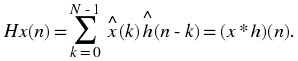
Hence, circular convolution has been defined such that the output of a linear time invariant system is given by the convolution of the system input with the system unit impulse response.
Graphical Intuition
It is often helpful to be able to visualize the computation of a circular convolution in terms of graphical processes. Consider the circular convolution of two finite length functions f,g given by
(4.29)
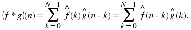
The first step in graphically understanding the operation of convolution is to plot each of the periodic extensions of the functions. Next, one of the functions must be selected, and its plot reflected across the k = 0 axis. For each k ∈ Z[0,N – 1], that same function must be shifted left by k . The product of the two resulting plots is then constructed. Finally, the area under the resulting curve on Z[0,N – 1] is computed.
Interactive Element
Figure 4.6.
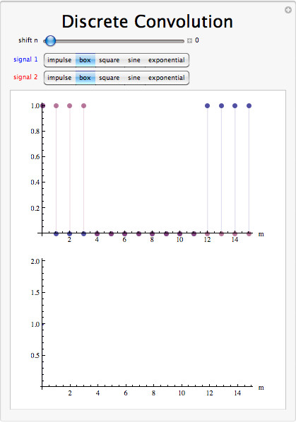
Interact (when online) with the Mathematica CDF demonstrating Discrete Linear Convolution. To download, right click and save file as .cdf
Convolution Summary
Convolution, one of the most important concepts in electrical engineering, can be used to determine the output signal of a linear time invariant system for a given input signal with knowledge of the system's unit impulse response. The operation of discrete time convolution is defined such that it performs this function for infinite length discrete time signals and systems. The operation of discrete time circular convolution is defined such that it performs this function for finite length and periodic discrete time signals. In each case, the output of the system is the convolution or circular convolution of the input signal with the unit impulse response.
4.4. Properties of Discrete Time Convolution*
Introduction
We have already shown the important role that discrete time convolution plays in signal processing. This section provides discussion and proof of some of the important properties of discrete time convolution. Analogous properties can be shown for discrete time circular convolution with trivial modification of the proofs provided except where explicitly noted otherwise.
Discrete Time Convolution Properties
Associativity
The operation of convolution is associative. That is, for all discrete time signals f 1,f 2,f 3 the following relationship holds.
(4.30)
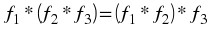
In order to show this, note that
(4.31)
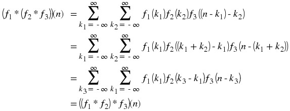
proving the relationship as desired through the substitution k 3 = k 1 + k 2 .
Commutativity
The operation of convolution is commutative. That is, for all discrete time signals f 1,f 2 the following relationship holds.
(4.32)f 1 * f 2 = f 2 * f 1
In order to show this, note that
(4.33)
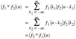
proving the relationship as desired through the substitution k 2 = n – k 1 .
Distribitivity
The operation of convolution is distributive over the operation of addition. That is, for all discrete time signals f 1,f 2,f 3 the following relationship holds.
(4.34)

In order to show this, note that
(4.35)
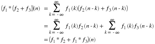
proving the relationship as desired.
Multilinearity
The operation of convolution is linear in each of the two function variables. Additivity in each variable results from distributivity of convolution over addition. Homogenity of order one in each varible results from the fact that for all discrete time signals f 1,f 2 and scalars a the following relationship holds.
(4.36)
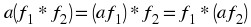
In order to show this, note that
(4.37)
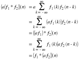
proving the relationship as desired.
Conjugation
The operation of convolution has the following property for all discrete time signals f 1,f 2 .
(4.38)
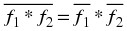
In order to show this, note that
(4.39)
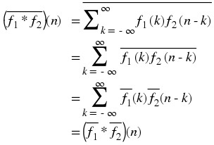
proving the relationship as desired.
Time Shift
The operation of convolution has the following property for all discrete time signals f 1,f 2 where S T is the time shift operator with T ∈ Z.
(4.40)

In order to show this, note that
(4.41)
proving the relationship as desired.
Impulse Convolution
The operation of convolution has the following property for all discrete time signals f where δ is the unit sample funciton.
(4.42)f * δ = f
In order to show this, note that
(4.43)
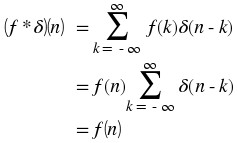
proving the relationship as desired.
Width
The operation of convolution has the following property for all discrete time signals f 1,f 2 where Duration(f) gives the duration of a signal f .
(4.44)

. In order to show this informally, note that  is nonzero for all n for which there is a k such that f
1(k)f
2(n – k) is nonzero. When viewing one function as reversed and sliding past the other, it is easy to see that such a k exists for all n on an interval of length
is nonzero for all n for which there is a k such that f
1(k)f
2(n – k) is nonzero. When viewing one function as reversed and sliding past the other, it is easy to see that such a k exists for all n on an interval of length 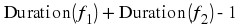 . Note that this is not always true of circular convolution of finite length and periodic signals as there is then a maximum possible duration within a period.
Convolution Properties Summary
As can be seen the operation of discrete time convolution has several important properties that have been listed and proven in this module. With silight modifications to proofs, most of these also extend to discrete time circular convolution as well and the cases in which exceptions occur have been noted above. These identities will be useful to keep in mind as the reader continues to study signals and systems.
4.5. Eigenfunctions of Discrete Time LTI Systems*
Introduction
Prior to reading this module, the reader should already have some experience with linear algebra and should specifically be familiar with the eigenvectors and eigenvalues of linear operators. A linear time invariant system is a linear operator defined on a function space that commutes with every time shift operator on that function space. Thus, we can also consider the eigenvector functions, or eigenfunctions, of a system. It is particularly easy to calculate the output of a system when an eigenfunction is the input as the output is simply the eigenfunction scaled by the associated eigenvalue. As will be shown, discrete time complex exponentials serve as eigenfunctions of linear time invariant systems operating on discrete time signals.
Eigenfunctions of LTI Systems
Consider a linear time invariant system H with impulse response h operating on some space of infinite length discrete time signals. Recall that the output H(x(n)) of the system for a given input x(n) is given by the discrete time convolution of the impulse response with the input
(4.45)

Now consider the input x(n) = e sn where s ∈ C. Computing the output for this input,
(4.46)
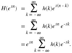
Thus,
(4.47)
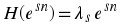
where
(4.48)
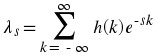
is the eigenvalue corresponding to the eigenvector e sn .
There are some additional points that should be mentioned. Note that, there still may be additional eigenvalues of a linear time invariant system not described by e sn for some s ∈ C. Furthermore, the above discussion has been somewhat formally loose as e sn may or may not belong to the space on which the system operates. However, for our purposes, complex exponentials will be accepted as eigenvectors of linear time invariant systems. A similar argument using discrete time circular convolution would also hold for spaces finite length signals.
Eigenfunction of LTI Systems Summary
As has been shown, discrete time complex exponential are eigenfunctions of linear time invariant systems operating on discrete time signals. Thus, it is particularly simple to calculate the output of a linear time invariant system for a complex exponential input as the result is a complex exponential output scaled by the associated eigenvalue. Consequently, representations of discrete time signals in terms of discrete time complex exponentials provide an advantage when studying signals. As will be explained later, this is what is accomplished by the discrete time Fourier transform and discrete time Fourier series, which apply to aperiodic and periodic signals respectively.
4.6. BIBO Stability of Discrete Time Systems*
Introduction
BIBO stability stands for bounded input, bounded output stability. BIBO stablity is the system property that any bounded input yields a bounded output. This is to say that as long as we input a signal with absolute value less than some constant, we are guaranteed to have an output with absolute value less than some other constant.
Discrete Time BIBO Stability
In order to understand this concept, we must first look more closely into exactly what we mean by bounded. A bounded signal is any signal such that there exists a value such that the absolute value of the signal is never greater than some value. Since this value is arbitrary, what we mean is that at no point can the signal tend to infinity, including the end behavior.
Figure 4.7.

A bounded signal is a signal for which there exists a constant A such that |f(t)| < A
Time Domain Conditions
Now that we have identified what it means for a signal to be bounded, we must turn our attention to the condition a system must possess in order to guarantee that if any bounded signal is passed through the system, a bounded signal will arise on the output. It turns out that a continuous-time LTI system with impulse response h(n) is BIBO stable if and only if it is absolutely summable. That is
(4.49)
Discrete-Time Condition for BIBO Stability
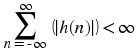
Z-Domain Conditions
Stability for discrete-time signals in the z-domain is about as easy to demonstrate as it is for continuous-time signals in the Laplace domain. However, instead of the region of convergence needing to contain the ⅈω -axis, the ROC must contain the unit circle. Consequently, for stable causal systems, all poles must be within the unit circle.
Figure 4.8.
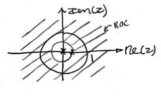
(a) A stable discrete-time system.
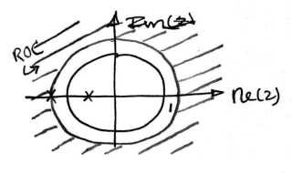
(b) An unstable discrete-time system.
BIBO Stability Summary
Bounded input bounded output stability, also known as BIBO stability, is an important and generally desirable system characteristic. A system is BIBO stable if every bounded input signal results in a bounded output signal, where boundedness is the property that the absolute value of a signal does not exceed some finite constant. In terms of time domain features, a discrete time system is BIBO stable if and only if its impulse response is absolutely summable. Equivalently, in terms of z-domain features, a continuous time system is BIBO stable if and only if the region of convergence of the transfer function includes the unit circle.
4.7. Linear Constant Coefficient Difference Equations*
Introduction: Difference Equations
In our study of signals and systems, it will often be useful to describe systems using equations involving the rate of change in some quantity. In discrete time, this is modeled through difference equations, which are a specific type of recurrance relation. For instance, recall that the funds in an account with discretely componded interest rate r will increase by r times the previous balance. Thus, a discretely compounded interest system is described by the first order difference equation shown in Equation 4.50.
(4.50)y ( n ) = ( 1 + r ) y ( n – 1 )
Given a sufficiently descriptive set of initial conditions or boundary conditions, if there is a solution to the difference equation, that solution is unique and describes the behavior of the system. Of course, the results are only accurate to the degree that the model mirrors reality.
Linear Constant Coefficient Difference Equations
An important subclass of difference equations is the set of linear constant coefficient difference equations. These equations are of the form
(4.51)C y ( n ) = f ( n )
where C is a difference operator of the form given
(4.52)C = c N D N + c N – 1 D N – 1 + . . . + c 1 D + c 0
in which D is the first difference operator
(4.53)D ( y ( n ) ) = y ( n ) – y ( n – 1 ) .
Note that operators of this type satisfy the linearity conditions, and c 0,...,c n are real constants.
However, Equation 4.51 can easily be written as a linear constant coefficient recurrence equation without difference operators. Conversely, linear constant coefficient recurrence equations can also be written in the form of a difference equation, so the two types of equations are different representations of the same relationship. Although we will still call them linear constant coefficient difference equations in this course, we typically will not write them using difference operators. Instead, we will write them in the simpler recurrence relation form
(4.54)
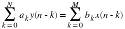
where x is the input to the system and y is the output. This can be rearranged to find y(n) as
(4.55)
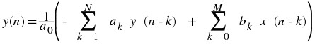
The forms provided by Equation 4.54 and Equation 4.55 will be used in the remainder of this course.
A similar concept for continuous time setting, differential equations, is discussed in the chapter on time domain analysis of continuous time systems. There are many parallels between the discussion of linear constant coefficient ordinary differential equations and linear constant coefficient differece equations.
Applications of Difference Equations
Difference equations can be used to describe many useful digital filters as described in the chapter discussing the z-transform. An additional illustrative example is provided here.
Example 4.4.
Recall that the Fibonacci sequence describes a (very unrealistic) model of what happens when a pair rabbits get left alone in a black box... The assumptions are that a pair of rabits never die and produce a pair of offspring every month starting on their second month of life. This system is defined by the recursion relation for the number of rabit pairs y(n) at month n
(4.56)y ( n ) = y ( n – 1 ) + y ( n – 2 )
with the initial conditions y(0) = 0 and y(1) = 1. The result is a very fast growth in the sequence. This is why we do not open black boxes.
Linear Constant Coefficient Difference Equations Summary
Difference equations are an important mathematical tool for modeling discrete time systems. An important subclass of these is the class of linear constant coefficient difference equations. Linear constant coefficient difference equations are often particularly easy to solve as will be described in the module on solutions to linear constant coefficient difference equations and are useful in describing a wide range of situations that arise in electrical engineering and in other fields.
4.8. Solving Linear Constant Coefficient Difference Equations*
Introduction
The approach to solving linear constant coefficient difference equations is to find the general form of all possible solutions to the equation and then apply a number of conditions to find the appropriate solution. The two main types of problems are initial value problems, which involve constraints on the solution at several consecutive points, and boundary value problems, which involve constraints on the solution at nonconsecutive points.
The number of initial conditions needed for an N th order difference equation, which is the order of the highest order difference or the largest delay parameter of the output in the equation, is N , and a unique solution is always guaranteed if these are supplied. Boundary value probelms can be slightly more complicated and will not necessarily have a unique solution or even a solution at all for a given set of conditions. Thus, this section will focus exclusively on initial value problems.
Solving Linear Constant Coefficient Difference Equations
Consider some linear constant coefficient difference equation given by A y(n) = f(n), in which A is a difference operator of the form
(4.57)A = a N D N + a N – 1 D N – 1 + . . . + a 1 D + a 0
where D is the first difference operator
(4.58)D ( y ( n ) ) = y ( n ) – y ( n – 1 ) .
Let y
h
(n) and y
p
(n) be two functions such that A
y
h
(n) = 0 and A
y
p
(n) = f(n). By the linearity of A , note that 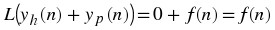 . Thus, the form of the general solution y
g
(n) to any linear constant coefficient ordinary differential equation is the sum of a homogeneous solution y
h
(n) to the equation A
y(n) = 0 and a particular solution y
p
(n) that is specific to the forcing function f(n).
. Thus, the form of the general solution y
g
(n) to any linear constant coefficient ordinary differential equation is the sum of a homogeneous solution y
h
(n) to the equation A
y(n) = 0 and a particular solution y
p
(n) that is specific to the forcing function f(n).
We wish to determine the forms of the homogeneous and nonhomogeneous solutions in full generality in order to avoid incorrectly restricting the form of the solution before applying any conditions. Otherwise, a valid set of initial or boundary conditions might appear to have no corresponding solution trajectory. The following sections discuss how to accomplish this for linear constant coefficient difference equations.
Finding the Homogeneous Solution
In order to find the homogeneous solution to a difference equation described by the recurrence relation ∑N k = 0 a k y(n – k) = f(n), consider the difference equation ∑N k = 0 a k y(n – k) = 0. We know that the solutions have the form c λ n for some complex constants c,λ . Since ∑N k = 0 a k c λ n – k = 0 for a solution it follows that
(4.59)
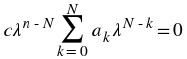
so it also follows that
(4.60)a 0 λ N + . . . + a N = 0 .
Therefore, the solution exponential are the roots of the above polynomial, called the characteristic polynomial.
For equations of order two or more, there will be several roots. If all of the roots are distinct, then the general form of the homogeneous solution is simply
(4.61)y h ( n ) = c 1 λ 1 n + . . . + c 2 λ 2 n .
If a root has multiplicity that is greater than one, the repeated solutions must be multiplied by each power of n from 0 to one less than the root multipicity (in order to ensure linearly independent solutions). For instance, if λ 1 had a multiplicity of 2 and λ 2 had multiplicity 3, the homogeneous solution would be
(4.62)y h ( n ) = c 1 λ 1 n + c 2 n λ 1 n + c 3 λ 2 n + c 4 n λ 2 n + c 5 n 2 λ 2 n .
Example 4.5.
Recall that the Fibonacci sequence describes a (very unrealistic) model of what happens when a pair rabbits get left alone in a black box... The assumptions are that a pair of rabits never die and produce a pair of offspring every month starting on their second month of life. This system is defined by the recursion relation for the number of rabit pairs y(n) at month n
(4.63)y ( n ) – y ( n – 1 ) – y ( n – 2 ) = 0
with the initial conditions y(0) = 0 and y(1) = 1.
Note that the forcing function is zero, so only the homogenous solution is needed. It is easy to see that the characteristic polynomial is λ 2 – λ – 1 = 0, so there are two roots with multiplicity one. These areand
. Thus, the solution is of the form
(4.64)
Using the initial conditions, we determine that
(4.65)

and
(4.66)

Hence, the Fibonacci sequence is given by
(4.67)
Finding the Particular Solution
Finding the particular solution is a slightly more complicated task than finding the homogeneous solution. It can be found through convolution of the input with the unit impulse response once the unit impulse response is known. Finding the particular solution ot a differential equation is discussed further in the chapter concerning the z-transform, which greatly simplifies the procedure for solving linear constant coefficient differential equations using frequency domain tools.
Example 4.6.
Consider the following difference equation describing a system with feedback
(4.68)y ( n ) – a y ( n – 1 ) = x ( n ) .
In order to find the homogeneous solution, consider the difference equation
(4.69)y ( n ) – a y ( n – 1 ) = 0 .
It is easy to see that the characteristic polynomial is λ – a = 0, so λ = a is the only root. Thus the homogeneous solution is of the form
(4.70)y h ( n ) = c 1 a n .
In order to find the particular solution, consider the output for the x(n) = δ(n) unit impulse case
(4.71)y ( n ) – a y ( n – 1 ) = δ ( n ) .
By inspection, it is clear that the impulse response is a n u(n). Hence, the particular solution for a given x(n) is
(4.72)y p ( n ) = x ( n ) * (a n u ( n ) ) .
Therefore, the general solution is
(4.73)y g ( n ) = y h ( n ) + y p ( n ) = c 1 a n + x ( n ) * (a n u ( n ) ) .
Initial conditions and a specific input can further tailor this solution to a specific situation.
Solving Difference Equations Summary
Linear constant coefficient difference equations are useful for modeling a wide variety of discrete time systems. The approach to solving them is to find the general form of all possible solutions to the equation and then apply a number of conditions to find the appropriate solution. This is done by finding the homogeneous solution to the difference equation that does not depend on the forcing function input and a particular solution to the difference equation that does depend on the forcing function input.
Chapter 5. Introduction to Fourier Analysis
Fourier's Daring Leap
Fourier postulated around 1807 that any periodic signal (equivalently finite length signal) can be built up as an infinite linear combination of harmonic sinusoidal waves.
i.e. Given the collection
(5.1)
any
(5.2)f ( t ) ∈ L 2 [ 0 , T )
can be approximated arbitrarily closely by
(5.3)
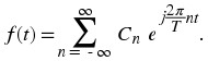
Now, The issue of exact convergence did bring Fourier much criticism from the French Academy of Science (Laplace, Lagrange, Monge and LaCroix comprised the review committee) for several years after its presentation on 1807. It was not resolved for also a century, and its resolution is interesting and important to understand from a practical viewpoint. See more in the section on Gibbs Phenomena.
Fourier analysis is fundamental to understanding the behavior of signals and systems. This is a result of the fact that sinusoids are Eigenfunctions of linear, time-invariant (LTI) systems. This is to say that if we pass any particular sinusoid through a LTI system, we get a scaled version of that same sinusoid on the output. Then, since Fourier analysis allows us to redefine the signals in terms of sinusoids, all we need to do is determine how any given system effects all possible sinusoids (its transfer function) and we have a complete understanding of the system. Furthermore, since we are able to define the passage of sinusoids through a system as multiplication of that sinusoid by the transfer function at the same frequency, we can convert the passage of any signal through a system from convolution (in time) to multiplication (in frequency). These ideas are what give Fourier analysis its power.
Now, after hopefully having sold you on the value of this method of analysis, we must examine exactly what we mean by Fourier analysis. The four Fourier transforms that comprise this analysis are the Fourier Series, Continuous-Time Fourier Transform, Discrete-Time Fourier Transform and Discrete Fourier Transform. For this document, we will view the Laplace Transform and Z-Transform as simply extensions of the CTFT and DTFT respectively. All of these transforms act essentially the same way, by converting a signal in time to an equivalent signal in frequency (sinusoids). However, depending on the nature of a specific signal i.e. whether it is finite- or infinite-length and whether it is discrete- or continuous-time) there is an appropriate transform to convert the signal into the frequency domain. Below is a table of the four Fourier transforms and when each is appropriate. It also includes the relevant convolution for the specified space.
| Transform | Time Domain | Frequency Domain | Convolution |
|---|---|---|---|
| Continuous-Time Fourier Series | L 2([0, T)) | l 2(ℤ) | Continuous-Time Circular |
| Continuous-Time Fourier Transform | L 2(ℝ) | L 2(ℝ) | Continuous-Time Linear |
| Discrete-Time Fourier Transform | l 2(ℤ) | L 2([0, 2π)) | Discrete-Time Linear |
| Discrete Fourier Transform | l 2([0, N − 1]) | l 2([0, N − 1]) | Discrete-Time Circular |
Chapter 6. Continuous Time Fourier Series (CTFS)
6.1. Continuous Time Periodic Signals*
Introduction
This module describes the type of signals acted on by the Continuous Time Fourier Series.
Relevant Spaces
The Continuous-Time Fourier Series maps finite-length (or T -periodic), continuous-time signals in L 2 to infinite-length, discrete-frequency signals in l 2 .
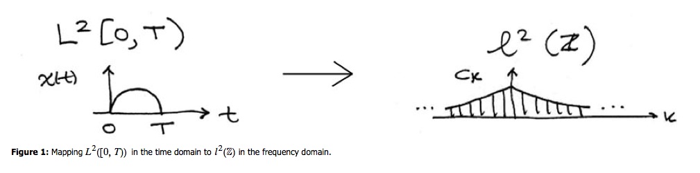
Periodic Signals
When a function repeats itself exactly after some given period, or cycle, we say it's periodic. A periodic function can be mathematically defined as: f(t) = f(t + mT) m ∈ ℤ where T > 0 represents the fundamental period of the signal, which is the smallest positive value of T for the signal to repeat. Because of this, you may also see a signal referred to as a T-periodic signal. Any function that satisfies this equation is said to be periodic with period T.
We can think of periodic functions (with period T ) two different ways:
as functions on all of ℝ
Figure 6.1.

Continuous time periodic function over all of ℝ where f(t 0) = f(t 0 + T)
or, we can cut out all of the redundancy, and think of them as functions on an interval
 (or, more generally,
  ). If we know the signal is T-periodic then all the information of the signal is captured by the above interval.
 Figure 6.2.
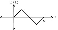
Remove the redundancy of the period function so that f(t) is undefined outside
 .
.
An aperiodic CT function f(t) , on the other hand, does not repeat for any T ∈ ℝ ; i.e. there exists no T such that this equation holds.
Demonstration
Here's an example demonstrating a periodic sinusoidal signal with various frequencies, amplitudes and phase delays:
Figure 6.3.
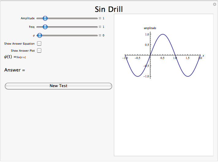
Interact (when online) with a Mathematica CDF demonstrating a Periodic Sinusoidal Signal with various frequencies, amplitudes, and phase delays. To download, right click and save file as .cdf.
To learn the full concept behind periodicity, see the video below.
Figure 6.4. Khan Lecture on Periodic Signals
(This media type is not supported in this reader. Click to open media in browser.)
video from Khan Academy
Conclusion
A periodic signal is completely defined by its values in one period, such as the interval [0,T].
6.2. Continuous Time Fourier Series (CTFS)*
Introduction
In this module, we will derive an expansion for continuous-time, periodic functions, and in doing so, derive the Continuous Time Fourier Series (CTFS).
Since complex exponentials are eigenfunctions of linear time-invariant (LTI) systems, calculating the output of an LTI system ℋ given ⅇ st as an input amounts to simple multiplication, where H(s) ∈ ℂ is the eigenvalue corresponding to s. As shown in the figure, a simple exponential input would yield the output y(t) = H(s)ⅇ st
Figure 6.5.
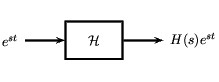
Simple LTI system.
Using this and the fact that ℋ is linear, calculating y(t) for combinations of complex exponentials is also straightforward.
c
1
ⅇ
s
1
t
+ c
2
ⅇ
s
2
t
→ c
1
H(s
1)ⅇ
s
1
t
+ c
2
H(s
2)ⅇ
s
2
t
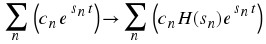
The action of H on an input such as those in the two equations above is easy to explain. ℋ independently scales each exponential component ⅇ s n t by a different complex number H(s n ) ∈ ℂ . As such, if we can write a function f(t) as a combination of complex exponentials it allows us to easily calculate the output of a system.
Fourier Series Synthesis
Joseph Fourier demonstrated that an arbitrary f(t) can be written as a linear combination of harmonic complex sinusoids  where
where  is the fundamental frequency. For almost all f(t) of practical interest, there exists c
n
to make Equation true. If f(t) is finite energy ( f(t) ∈ L
2[0, T] ), then the equality in Equation holds in the sense of energy convergence; if f(t) is continuous, then Equation holds pointwise. Also, if f(t) meets some mild conditions (the Dirichlet conditions), then Equation holds pointwise everywhere except at points of discontinuity.
is the fundamental frequency. For almost all f(t) of practical interest, there exists c
n
to make Equation true. If f(t) is finite energy ( f(t) ∈ L
2[0, T] ), then the equality in Equation holds in the sense of energy convergence; if f(t) is continuous, then Equation holds pointwise. Also, if f(t) meets some mild conditions (the Dirichlet conditions), then Equation holds pointwise everywhere except at points of discontinuity.
The c n - called the Fourier coefficients - tell us "how much" of the sinusoid ⅇ j ω 0 n t is in f(t) . The formula shows f(t) as a sum of complex exponentials, each of which is easily processed by an LTI system (since it is an eigenfunction of every LTI system). Mathematically, it tells us that the set of complex exponentials {ⅇ j ω 0 n t , n ∈ ℤ } form a basis for the space of T-periodic continuous time functions.
Example 6.1.
We know from Euler's formula that
Synthesis with Sinusoids Demonstration
Figure 6.6.
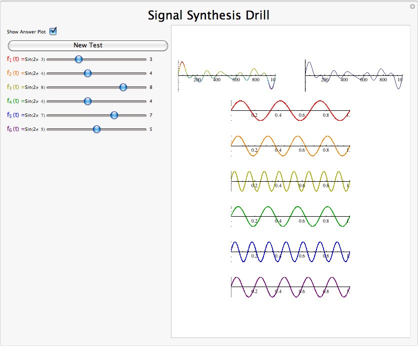
Interact(when online) with a Mathematica CDF demonstrating sinusoid synthesis. To download, right click and save as .cdf.
Figure 6.7. Guitar Oscillations on an iPhone
(This media type is not supported in this reader. Click to open media in browser.)
Fourier Series Analysis
Finding the coefficients of the Fourier series expansion involves some algebraic manipulation of the synthesis formula. First of all we will multiply both sides of the equation by ⅇ
– (j
ω
0
k
t) , where k ∈ ℤ .  Now integrate both sides over a given period, T :
 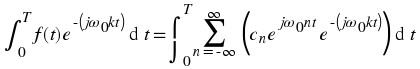 On the right-hand side we can switch the summation and integral and factor the constant out of the integral.
 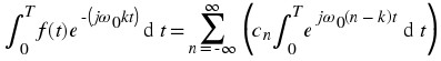 Now that we have made this seemingly more complicated, let us focus on just the integral,
 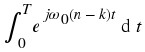 , on the right-hand side of the above equation. For this integral we will need to consider two cases: n = k and n ≠ k . For n = k we will have:
 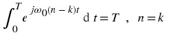 For n ≠ k , we will have:
  But cos(ω
0(n − k)t) has an integer number of periods, n − k , between 0 and T . Imagine a graph of the cosine; because it has an integer number of periods, there are equal areas above and below the x-axis of the graph. This statement holds true for sin(ω
0(n − k)t) as well. What this means is
But cos(ω
0(n − k)t) has an integer number of periods, n − k , between 0 and T . Imagine a graph of the cosine; because it has an integer number of periods, there are equal areas above and below the x-axis of the graph. This statement holds true for sin(ω
0(n − k)t) as well. What this means is 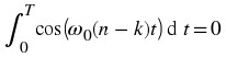 which also holds for the integral involving the sine function. Therefore, we conclude the following about our integral of interest:
 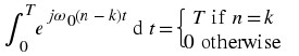 Now let us return our attention to our complicated equation, Equation, to see if we can finish finding an equation for our Fourier coefficients. Using the facts that we have just proven above, we can see that the only time Equation will have a nonzero result is when k and n are equal:
 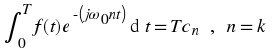 Finally, we have our general equation for the Fourier coefficients:
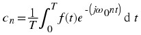
Example 6.2.
Consider the square wave function given by
(6.1)
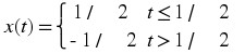
on the unit interval t ∈ Z[0,1).
(6.2)
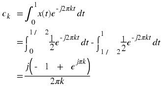
Thus, the Fourier coefficients of this function found using the Fourier series analysis formula are
(6.3)
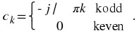
Fourier Series Summary
Because complex exponentials are eigenfunctions of LTI systems, it is often useful to represent signals using a set of complex exponentials as a basis. The continuous time Fourier series synthesis formula expresses a continuous time, periodic function as the sum of continuous time, discrete frequency complex exponentials. 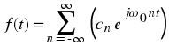 The continuous time Fourier series analysis formula gives the coefficients of the Fourier series expansion.
  In both of these equations
  is the fundamental frequency.
6.3. Common Fourier Series*
Introduction
Once one has obtained a solid understanding of the fundamentals of Fourier series analysis and the General Derivation of the Fourier Coefficients, it is useful to have an understanding of the common signals used in Fourier Series Signal Approximation.
Deriving the Fourier Coefficients
Consider a square wave f(x) of length 1. Over the range [0,1), this can be written as 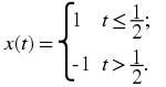
Figure 6.8. Fourier series approximation of a square wave
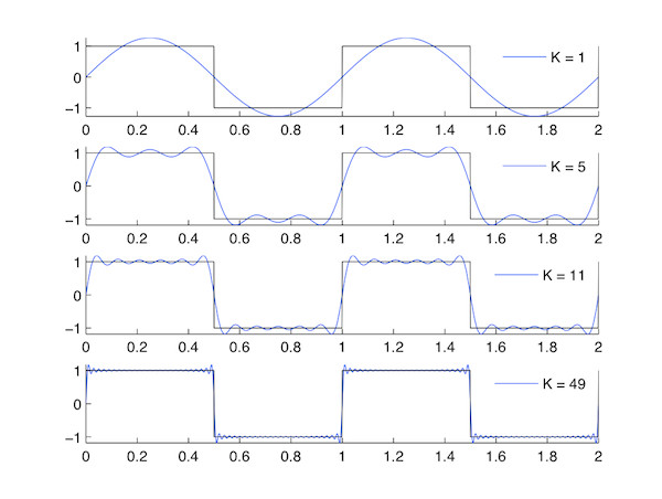
Fourier series approximation to sq(t) . The number of terms in the Fourier sum is indicated in each plot, and the square wave is shown as a dashed line over two periods.
Real Even Signals
Given that the square wave is a real and even signal,
f(t) = f( – t) EVEN
f(t) = f *(t) REAL
therefore,
c n = c – n EVEN
c n = c n * REAL
Consider this mathematical question intuitively: Can a discontinuous function, like the square wave, be expressed as a sum, even an infinite one, of continuous signals? One should at least be suspicious, and in fact, it can't be thus expressed.
The extraneous peaks in the square wave's Fourier series never disappear; they are termed Gibb's phenomenon after the American physicist Josiah Willard Gibbs. They occur whenever the signal is discontinuous, and will always be present whenever the signal has jumps.
Deriving the Fourier Coefficients for Other Signals
The Square wave is the standard example, but other important signals are also useful to analyze, and these are included here.
Constant Waveform
This signal is relatively self-explanatory: the time-varying portion of the Fourier Coefficient is taken out, and we are left simply with a constant function over all time. x ( t ) = 1
Sinusoid Waveform
With this signal, only a specific frequency of time-varying Coefficient is chosen (given that the Fourier Series equation includes a sine wave, this is intuitive), and all others are filtered out, and this single time-varying coefficient will exactly match the desired signal. x ( t ) = s i n ( π t )
Triangle Waveform
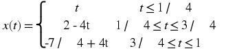 This is a more complex form of signal approximation to the square wave. Because of the Symmetry Properties of the Fourier Series, the triangle wave is a real and odd signal, as opposed to the real and even square wave signal. This means that
f(t) = – f( – t) ODD
f(t) = f *(t) REAL
therefore,
c n = – c – n
c n = – c n * IMAGINARY
Figure 6.9. Fourier series approximation of a triangle wave
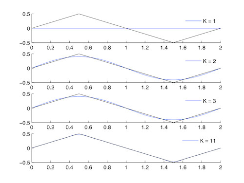
Sawtooth Waveform
x ( t ) = t – F l o o r ( t ) Because of the Symmetry Properties of the Fourier Series, the sawtooth wave can be defined as a real and odd signal, as opposed to the real and even square wave signal. This has important implications for the Fourier Coefficients.
Figure 6.10. Fourier series approximation of a sawtooth wave
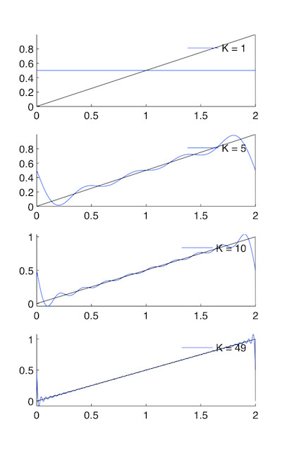
Fourier Series Approximation VI
Figure 6.11.
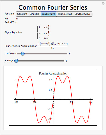
Interact (when online) with a Mathematica CDF demonstrating the common Fourier Series. To download, right click and save file as .cdf.
link: http://yoder-3.institute.rose-hulman.edu/visible3/chapters/03spect/demosLV/fseries/index.htm
Summary
To summarize, a great deal of variety exists among the common Fourier Transforms. A summary table is provided here with the essential information.
| Description | Time Domain Signal for t ∈ [0,1) | Frequency Domain Signal |
| Constant Waveform | x ( t ) = 1 | 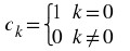
|
| Sinusoid Waveform | x ( t ) = s i n ( π t ) | 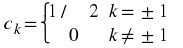
|
| Square Waveform | 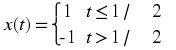
| 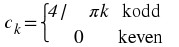
|
| Triangle Waveform | 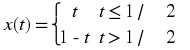
| 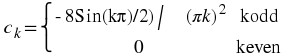
|
| Sawtooth Waveform | x ( t ) = t / 2 | 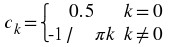
|
6.4. Properties of the CTFS*
Introduction
In this module we will discuss the basic properties of the Continuous-Time Fourier Series. We will begin by refreshing your memory of our basic Fourier series equations: 
 Let ℱ{·} denote the transformation from f(t) to the Fourier coefficients ℱ{f(t)} = c
n
, n ∈ ℤ ℱ{·} maps complex valued functions to sequences of complex numbers.
Let ℱ{·} denote the transformation from f(t) to the Fourier coefficients ℱ{f(t)} = c
n
, n ∈ ℤ ℱ{·} maps complex valued functions to sequences of complex numbers.
Linearity
ℱ{·} is a linear transformation.
Theorem 6.1.
If ℱ{f(t)} = c n and ℱ{g(t)} = d n . Then ℱ{α f(t)} = α c n , α ∈ ℂ and ℱ{f(t) + g(t)} = c n + d n
Proof
Easy. Just linearity of integral. 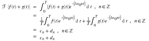
Shifting
Shifting in time equals a phase shift of Fourier coefficients
Theorem 6.2.
ℱ{f(t − t 0)} = ⅇ – (ⅈ ω 0 n t 0) c n if c n = |c n |ⅇ ⅈ∠c n , then |ⅇ – (ⅈ ω 0 n t 0) c n | = |ⅇ – (ⅈ ω 0 n t 0)||c n | = |c n | ∠ⅇ – (ⅈ ω 0 t 0 n) = ∠c n − ω 0 t 0 n
Proof
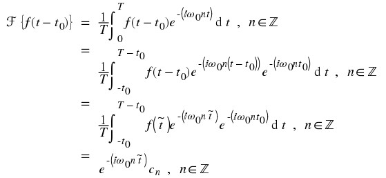
Parseval's Relation
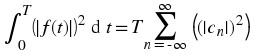 Parseval's relation tells us that the energy of a signal is equal to the energy of its Fourier transform.
Note
Parseval tells us that the Fourier series maps L 2([0, T]) to l 2(ℤ) .
Figure 6.12.
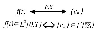
Exercise 6.4.1. (Go to Solution)
For f(t) to have "finite energy," what do the c n do as n → ∞ ?
Exercise 6.4.2. (Go to Solution)
If  , is f ∈ L
2([0, T]) ?
, is f ∈ L
2([0, T]) ?
Exercise 6.4.3. (Go to Solution)
Now, if  , is f ∈ L
2([0, T]) ?
, is f ∈ L
2([0, T]) ?
The rate of decay of the Fourier series determines if f(t) has finite energy.
Parsevals Theorem Demonstration
Figure 6.13.

Interact (when online) with a Mathematica CDF demonstrating Parsevals Theorem. To download, right click and save file as .cdf.
Symmetry Properties
Rule 6.1. Even Signals
Even Signals
f(t) = f( – t)
∥ c n ∥ = ∥ c – n ∥
Proof


Rule 6.2. Odd Signals
Odd Signals
f ( t ) = -f ( -t )
c n = c – n *
Proof

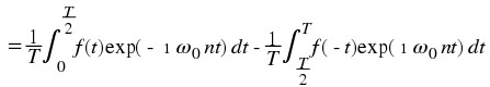
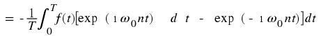
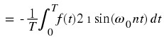
Rule 6.3. Real Signals
Real Signals
f(t) = f *(t)
c n = c – n *
Proof


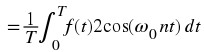
Differentiation in Fourier Domain
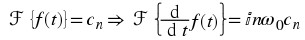
Since 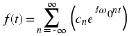 then
then 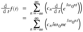 A differentiator attenuates the low frequencies in f(t) and accentuates the high frequencies. It removes general trends and accentuates areas of sharp variation.
Note
A common way to mathematically measure the smoothness of a function f(t) is to see how many derivatives are finite energy.
This is done by looking at the Fourier coefficients of the signal, specifically how fast they decay as n → ∞ . If ℱ{f(t)} = c
n
and |c
n
| has the form  , then
 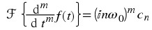 and has the form
  . So for the m
th derivative to have finite energy, we need
. So for the m
th derivative to have finite energy, we need  thus
thus  decays faster than
  which implies that 2k − 2m > 1 or
  Thus the decay rate of the Fourier series dictates smoothness.
Fourier Differentiation Demonstration
Figure 6.14.
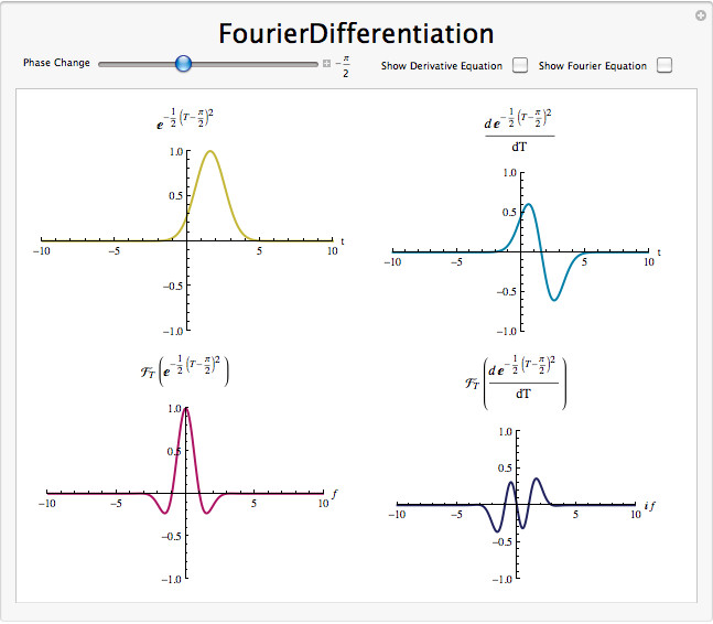
Interact (when online) with a Mathematica CDF demonstrating Differentiation in the Fourier Domain. To download, right click and save file as .cdf.
Integration in the Fourier Domain
If ℱ{f(t)} = c
n
then 
Note
If c 0 ≠ 0 , this expression doesn't make sense.
Integration accentuates low frequencies and attenuates high frequencies. Integrators bring out the general trends in signals and suppress short term variation (which is noise in many cases). Integrators are much nicer than differentiators.
Fourier Integration Demonstration
Figure 6.15.

Interact (when online) with a Mathematica CDF demonstrating Integration in the Fourier Domain. To download, right click and save file as .cdf.
Signal Multiplication and Convolution
Given a signal f(t) with Fourier coefficients c
n
and a signal g(t) with Fourier coefficients d
n
, we can define a new signal, y(t) , where y(t) = f(t)g(t) . We find that the Fourier Series representation of y(t) , e
n
, is such that  . This is to say that signal multiplication in the time domain is equivalent to signal convolution in the frequency domain, and vice-versa: signal multiplication in the frequency domain is equivalent to signal convolution in the time domain. The proof of this is as follows
 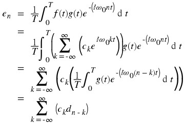 for more details, see the section on Signal convolution and the CTFS
Conclusion
Like other Fourier transforms, the CTFS has many useful properties, including linearity, equal energy in the time and frequency domains, and analogs for shifting, differentation, and integration.
| Property | Signal | CTFS |
| Linearity | a x ( t ) + b y ( t ) | a X ( f ) + b Y ( f ) |
| Time Shifting | x ( t – τ ) | X ( f ) e – j 2 π f τ / T |
| Time Modulation | x ( t ) e j 2 π f τ / T | X ( f – k ) |
| Multiplication | x ( t ) y ( t ) | X ( f ) * Y ( f ) |
| Continuous Convolution | x ( t ) * y ( t ) | X ( f ) Y ( f ) |
Solutions to Exercises
Solution to Exercise 6.4.1. (Return to Exercise)
(|c n |)2 < ∞ for f(t) to have finite energy.
Solution to Exercise 6.4.2. (Return to Exercise)
Yes, because  , which is summable.
Solution to Exercise 6.4.3. (Return to Exercise)
No, because  , which is not summable.
6.5. Continuous Time Circular Convolution and the CTFS*
Introduction
This module relates circular convolution of periodic signals in the time domain to multiplication in the frequency domain.
Signal Circular Convolution
Given a signal f(t) with Fourier coefficients c
n
and a signal g(t) with Fourier coefficients d
n
, we can define a new signal, v(t) , where v(t) = (f(t) ⊛ g(t)) We find that the Fourier Series representation of v(t) , a
n
, is such that a
n
= c
n
d
n
. (f(t) ⊛ g(t)) is the circular convolution of two periodic signals and is equivalent to the convolution over one interval, i.e.
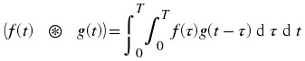 .
.
Note
Circular convolution in the time domain is equivalent to multiplication of the Fourier coefficients.
This is proved as follows 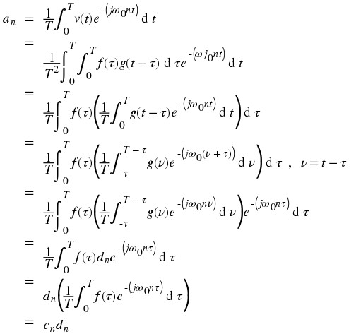
Exercise
Take a look at a square pulse with a period of T.
Figure 6.16.
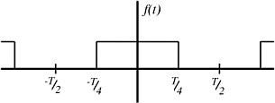
For this signal 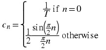
Take a look at a triangle pulse train with a period of T.
Figure 6.17.
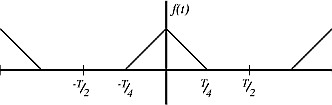
This signal is created by circularly convolving the square pulse with itself. The Fourier coefficients for this signal are 
Exercise 6.5.1. (Go to Solution)
Find the Fourier coefficients of the signal that is created when the square pulse and the triangle pulse are convolved.
Conclusion
Circular convolution in the time domain is equivalent to multiplication of the Fourier coefficients in the frequency domain.
Solutions to Exercises
Solution to Exercise 6.5.1. (Return to Exercise)
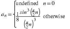
6.6. Convergence of Fourier Series*
TODO
ADD AUTHOR/MAINTAINER/CRHOLDER: Ricardo Radaelli-Sanchez MODULE ID: m10089
Introduction
Before looking at this module, hopefully you have become fully convinced of the fact that any
periodic function, f(t) , can be represented as a sum of complex sinusoids. If you are not, then try looking back at eigen-stuff in a nutshell or eigenfunctions of LTI systems. We have shown that we can represent a signal as the sum of exponentials through the Fourier Series equations below: 
 Joseph Fourier insisted that these equations were true, but could not prove it. Lagrange publicly ridiculed Fourier, and said that only continuous functions can be represented by Equation (indeed he proved that Equation holds for continuous-time functions). However, we know now that the real truth lies in between Fourier and Lagrange's positions.
Understanding the Truth
Formulating our question mathematically, let 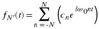 where c
n
equals the Fourier coefficients of f(t) (see Equation).
where c
n
equals the Fourier coefficients of f(t) (see Equation).
f
N
′(t) is a "partial reconstruction" of f(t) using the first 2N + 1 Fourier coefficients. f
N
′(t) approximates
f(t) , with the approximation getting better and better as N gets large. Therefore, we can think of the set  as a sequence of functions, each one approximating f(t) better than the one before.
The question is, does this sequence converge to f(t) ? Does f N ′(t) → f(t) as N → ∞ ? We will try to answer this question by thinking about convergence in two different ways:
Looking at the energy of the error signal: e N (t) = f(t) − f N ′(t)
Looking at
 at each point and comparing to f(t) .
Approach #1
Let e
N
(t) be the difference (i.e. error) between the signal f(t) and its partial reconstruction f
N
′(t) e
N
(t) = f(t) − f
N
′(t) If  (finite energy), then the energy of e
N
(t) → 0 as N → ∞ is
(finite energy), then the energy of e
N
(t) → 0 as N → ∞ is  We can prove this equation using Parseval's relation:
  where the last equation before zero is the tail sum of the Fourier Series, which approaches zero because
  . Since physical systems respond to energy, the Fourier Series provides an adequate representation for all
  equaling finite energy over one period.
Approach #2
The fact that e
N
→ 0 says nothing about f(t) and  being equal at a given point. Take the two functions graphed below for example:
Figure 6.18.
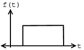
(a)
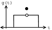
(b)
Given these two functions, f(t) and g(t) , then we can see that for all t , f(t) ≠ g(t) , but  From this we can see the following relationships: energy convergence ≠ pointwise convergence
  However, the reverse of the above statement does not hold true.
It turns out that if f(t) has a discontinuity (as can be seen in figure of g(t) above) at t
0 , then  But as long as f(t) meets some other fairly mild conditions, then
  if f(t) is continuous at t = t
′
.These conditions are known as the Dirichlet Conditions.
if f(t) is continuous at t = t
′
.These conditions are known as the Dirichlet Conditions.
Dirichlet Conditions
Named after the German mathematician, Peter Dirichlet, the Dirichlet conditions are the sufficient conditions to guarantee existence and energy convergence of the Fourier Series.
The Weak Dirichlet Condition for the Fourier Series
For the Fourier Series to exist, the Fourier coefficients must be finite. The Weak Dirichlet Condition guarantees this. It essentially says that the integral of the absolute value of the signal must be finite.
Theorem 6.3.
The coefficients of the Fourier Series are finite if
(6.4)
Weak Dirichlet Condition for the Fourier Series
Proof
This can be shown from the magnitude of the Fourier Series coefficients: 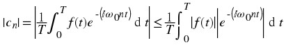 Remembering our complex exponentials, we know that in the above equation |ⅇ
– (ⅈ
ω
0
n
t)| = 1 , which gives us:
Remembering our complex exponentials, we know that in the above equation |ⅇ
– (ⅈ
ω
0
n
t)| = 1 , which gives us: 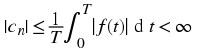

Note
If we have the function:then you should note that this function fails the above condition because:
The Strong Dirichlet Conditions for the Fourier Series
For the Fourier Series to exist, the following two conditions must be satisfied (along with the Weak Dirichlet Condition):
In one period, f(t) has only a finite number of minima and maxima.
In one period, f(t) has only a finite number of discontinuities and each one is finite.
These are what we refer to as the Strong Dirichlet Conditions. In theory we can think of signals that violate these conditions, sin(logt) for instance. However, it is not possible to create a signal that violates these conditions in a lab. Therefore, any real-world signal will have a Fourier representation.
Example 6.3.
Let us assume we have the following function and equality:If f(t) meets all three conditions of the Strong Dirichlet Conditions, then f(τ) = f ′(τ) at every τ at which f(t) is continuous. And where f(t) is discontinuous, f ′(t) is the average of the values on the right and left.
Figure 6.19.
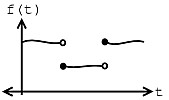
(a)
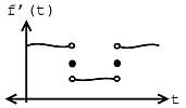
(b)
Discontinuous functions, f(t) .
Note
The functions that fail the strong Dirchlet conditions are pretty pathological - as engineers, we are not too interested in them.
6.7. Gibbs Phenomena*
Introduction
The Fourier Series is the representation of continuous-time, periodic signals in terms of complex exponentials. The Dirichlet conditions suggest that discontinuous signals may have a Fourier Series representation so long as there are a finite number of discontinuities. This seems counter-intuitive, however, as complex exponentials are continuous functions. It does not seem possible to exactly reconstruct a discontinuous function from a set of continuous ones. In fact, it is not. However, it can be if we relax the condition of 'exactly' and replace it with the idea of 'almost everywhere'. This is to say that the reconstruction is exactly the same as the original signal except at a finite number of points. These points, not necessarily surprisingly, occur at the points of discontinuities.
History
In the late 1800s, many machines were built to calculate Fourier coefficients and re-synthesize:  Albert Michelson (an extraordinary experimental physicist) built a machine in 1898 that could compute c
n
up to n = ± 79 , and he re-synthesized
Albert Michelson (an extraordinary experimental physicist) built a machine in 1898 that could compute c
n
up to n = ± 79 , and he re-synthesized 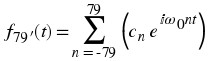 The machine performed very well on all tests except those involving discontinuous functions. When a square wave, like that shown in Figure 6.20, was inputed into the machine, "wiggles" around the discontinuities appeared, and even as the number of Fourier coefficients approached infinity, the wiggles never disappeared - these can be seen in the last plot in Figure 6.20. J. Willard Gibbs first explained this phenomenon in 1899, and therefore these discontinuous points are referred to as Gibbs Phenomenon.
Explanation
We begin this discussion by taking a signal with a finite number of discontinuities (like a square pulse) and finding its Fourier Series representation. We then attempt to reconstruct it from these Fourier coefficients. What we find is that the more coefficients we use, the more the signal begins to resemble the original. However, around the discontinuities, we observe rippling that does not seem to subside. As we consider even more coefficients, we notice that the ripples narrow, but do not shorten. As we approach an infinite number of coefficients, this rippling still does not go away. This is when we apply the idea of almost everywhere. While these ripples remain (never dropping below 9% of the pulse height), the area inside them tends to zero, meaning that the energy of this ripple goes to zero. This means that their width is approaching zero and we can assert that the reconstruction is exactly the original except at the points of discontinuity. Since the Dirichlet conditions assert that there may only be a finite number of discontinuities, we can conclude that the principle of almost everywhere is met. This phenomenon is a specific case of nonuniform convergence.
Below we will use the square wave, along with its Fourier Series representation, and show several figures that reveal this phenomenon more mathematically.
Square Wave
The Fourier series representation of a square signal below says that the left and right sides are "equal." In order to understand Gibbs Phenomenon we will need to redefine the way we look at equality. 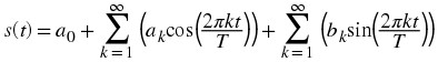
Example 6.4.
Figure 1 shows several Fourier series approximations of the square wave using a varied number of terms, denoted by K :
Figure 6.20. Fourier series approximations of a square wave
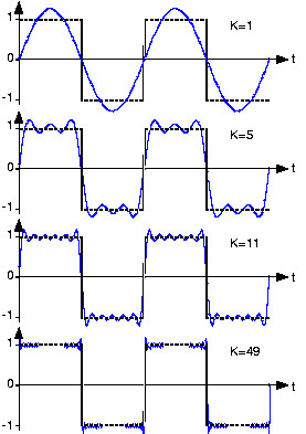
Fourier series approximation to sq(t) . The number of terms in the Fourier sum is indicated in each plot, and the square wave is shown as a dashed line over two periods.
When comparing the square wave to its Fourier series representation in Figure 6.20, it is not clear that the two are equal. The fact that the square wave's Fourier series requires more terms for a given representation accuracy is not important. However, close inspection of Figure 6.20 does reveal a potential issue: Does the Fourier series really equal the square wave at all values of t ? In particular, at each step-change in the square wave, the Fourier series exhibits a peak followed by rapid oscillations. As more terms are added to the series, the oscillations seem to become more rapid and smaller, but the peaks are not decreasing. Consider this mathematical question intuitively: Can a discontinuous function, like the square wave, be expressed as a sum, even an infinite one, of continuous ones? One should at least be suspicious, and in fact, it can't be thus expressed. This issue brought Fourier much criticism from the French Academy of Science (Laplace, Legendre, and Lagrange comprised the review committee) for several years after its presentation on 1807. It was not resolved for also a century, and its resolution is interesting and important to understand from a practical viewpoint.
The extraneous peaks in the square wave's Fourier series never disappear; they are termed Gibb's phenomenon after the American physicist Josiah Willard Gibbs. They occur whenever the signal is discontinuous, and will always be present whenever the signal has jumps.
Redefine Equality
Let's return to the question of equality; how can the equal sign in the definition of the Fourier series be justified? The partial answer is that pointwise--each and every value of t --equality is not guaranteed. What mathematicians later in the nineteenth century showed was that the rms error of the Fourier series was always zero.  What this means is that the difference between an actual signal and its Fourier series representation may not be zero, but the square of this quantity has zero integral! It is through the eyes of the rms value that we define equality: Two signals s
1(t) , s
2(t) are said to be equal in the mean square if rms(s
1 − s
2) = 0 . These signals are said to be equal pointwise if s
1(t) = s
2(t) for all values of t . For Fourier series, Gibb's phenomenon peaks have finite height and zero width: The error differs from zero only at isolated points--whenever the periodic signal contains discontinuities--and equals about 9% of the size of the discontinuity. The value of a function at a finite set of points does not affect its integral. This effect underlies the reason why defining the value of a discontinuous function at its discontinuity is meaningless. Whatever you pick for a value has no practical relevance for either the signal's spectrum or for how a system responds to the signal. The Fourier series value "at" the discontinuity is the average of the values on either side of the jump.
What this means is that the difference between an actual signal and its Fourier series representation may not be zero, but the square of this quantity has zero integral! It is through the eyes of the rms value that we define equality: Two signals s
1(t) , s
2(t) are said to be equal in the mean square if rms(s
1 − s
2) = 0 . These signals are said to be equal pointwise if s
1(t) = s
2(t) for all values of t . For Fourier series, Gibb's phenomenon peaks have finite height and zero width: The error differs from zero only at isolated points--whenever the periodic signal contains discontinuities--and equals about 9% of the size of the discontinuity. The value of a function at a finite set of points does not affect its integral. This effect underlies the reason why defining the value of a discontinuous function at its discontinuity is meaningless. Whatever you pick for a value has no practical relevance for either the signal's spectrum or for how a system responds to the signal. The Fourier series value "at" the discontinuity is the average of the values on either side of the jump.
Visualizing Gibb's Phenomena
The following VI demonstrates the occurrence of Gibb's Phenomena. Note how the wiggles near the square pulse to the left remain even if you drastically increase the order of the approximation, even though they do become narrower. Also notice how the approximation of the smooth region in the middle is much better than that of the discontinuous region, especially at lower orders.
Figure 6.21.
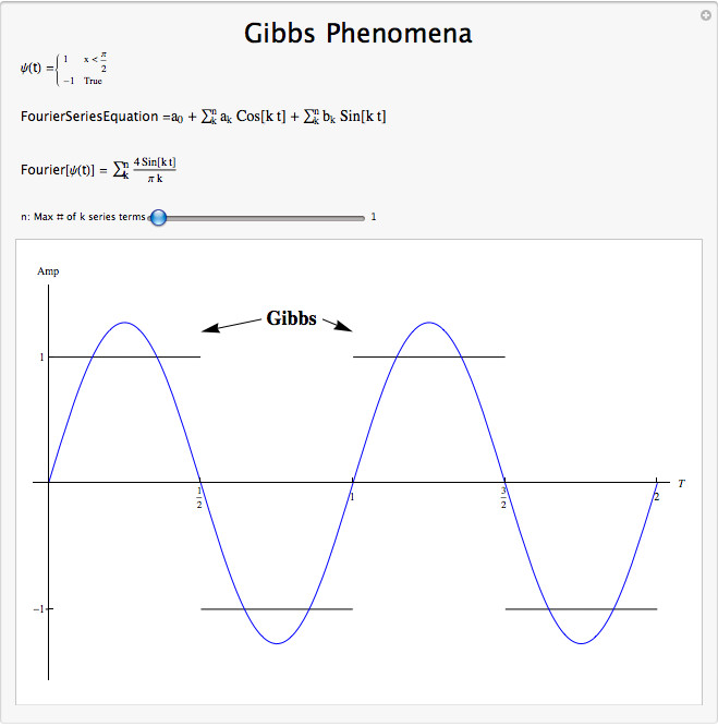
Interact (when online) with a Mathematica CDF demonstrating Gibbs Phenomena. To download, right click and save as .cdf.
Conclusion
We can approximate a function by re-synthesizing using only some of the Fourier coefficients (truncating the F.S.)  This approximation works well where f(t) is continuous, but not so well where f(t) is discontinuous. In the regions of discontinuity, we will always find Gibb's Phenomena, which never decrease below 9% of the height of the discontinuity, but become narrower and narrower as we add more terms.
Chapter 7. Discrete Time Fourier Series (DTFS)
7.1. Discrete Time Periodic Signals*
Introduction
This module describes the type of signals acted on by the Discrete Time Fourier Series.
Relevant Spaces
The Discrete Time Fourier Series maps finite-length (or N -periodic), discrete time signals in L 2 to finite-length, discrete-frequency signals in l 2 .
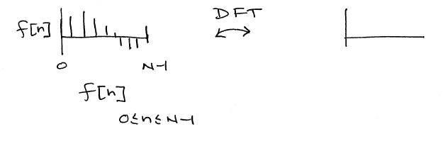
Periodic signals in discrete time repeats themselves in each cycle. However, only integers are allowed as time variable in discrete time. We denote signals in such case as x[n], n = ..., -2, -1, 0, 1, 2, ...
Periodic Signals
When a function repeats itself exactly after some given period, or cycle, we say it's periodic. A periodic function can be mathematically defined as: f[n] = f[n + mN] m ∈ ℤ where N > 0 represents the fundamental period of the signal, which is the smallest positive value of N for the signal to repeat. Because of this, you may also see a signal referred to as an N-periodic signal. Any function that satisfies this equation is said to be periodic with period N. Here's an example of a discrete-time periodic signal with period N:
Figure 7.1. discrete-time periodic signal

Notice the function is the same after a time shift of N
We can think of periodic functions (with period N ) two different ways:
as functions on all of ℝ
Figure 7.2.

discrete time periodic function over all of ℝ where f[n 0] = f[n 0 + N]
or, we can cut out all of the redundancy, and think of them as functions on an interval
 (or, more generally,
  ). If we know the signal is N-periodic then all the information of the signal is captured by the above interval.
 Figure 7.3.

Remove the redundancy of the period function so that f[n] is undefined outside
 .
.
An aperiodic DT function f[n] does not repeat for any N ∈ ℝ ; i.e. there exists no N such that this equation holds.
SinDrillDiscrete Demonstration
Here's an example demonstrating a periodic sinusoidal signal with various frequencies, amplitudes and phase delays:
Figure 7.4.
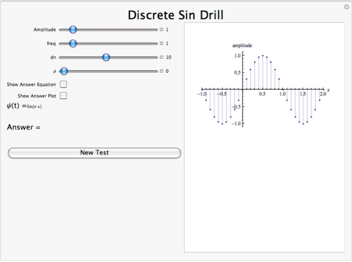
Interact (when online) with a Mathematica CDF demonstrating a discrete periodic sinusoidal signal with various frequencies, amplitudes and phase delays.
Conclusion
A discrete periodic signal is completely defined by its values in one period, such as the interval [0,N].
7.2. Discrete Time Fourier Series (DTFS)*
Introduction
In this module, we will derive an expansion for discrete-time, periodic functions, and in doing so, derive the Discrete Time Fourier Series (DTFS), or the Discrete Fourier Transform (DFT).
DTFS
Eigenfunction analysis
Since complex exponentials are eigenfunctions of linear time-invariant (LTI) systems, calculating the output of an LTI system ℋ given ⅇ
ⅈωn
as an input amounts to simple multiplication, where  , and where H[k] ∈ ℂ is the eigenvalue corresponding to k. As shown in the figure, a simple exponential input would yield the output y[n] = H[k]ⅇ
ⅈωn
, and where H[k] ∈ ℂ is the eigenvalue corresponding to k. As shown in the figure, a simple exponential input would yield the output y[n] = H[k]ⅇ
ⅈωn
Figure 7.5.

Simple LTI system.
Using this and the fact that ℋ is linear, calculating y[n] for combinations of complex exponentials is also straightforward.
c
1
ⅇ
ⅈ
ω
1
n
+ c
2
ⅇ
ⅈ
ω
2
n
→ c
1
H[k
1]ⅇ
ⅈ
ω
1
n
+ c
2
H[k
2]ⅇ
ⅈ
ω
1
n
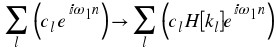
The action of H on an input such as those in the two equations above is easy to explain. ℋ independently scales each exponential component ⅇ ⅈ ω l n by a different complex number H[k l ] ∈ ℂ . As such, if we can write a function y[n] as a combination of complex exponentials it allows us to easily calculate the output of a system.
DTFS synthesis
It can be demonstrated that an arbitrary Discrete Time-periodic function
f[n] can be written as a linear combination of harmonic complex sinusoids  where
where  is the fundamental frequency. For almost all f[n] of practical interest, there exists c
n
to make Equation true. If f[n] is finite energy ( f[n] ∈ L
2[0, N] ), then the equality in Equation holds in the sense of energy convergence; with discrete-time signals, there are no concerns for divergence as there are with continuous-time signals.
is the fundamental frequency. For almost all f[n] of practical interest, there exists c
n
to make Equation true. If f[n] is finite energy ( f[n] ∈ L
2[0, N] ), then the equality in Equation holds in the sense of energy convergence; with discrete-time signals, there are no concerns for divergence as there are with continuous-time signals.
The c n - called the Fourier coefficients - tell us "how much" of the sinusoid ⅇ j ω 0 k n is in f[n] . The formula shows f[n] as a sum of complex exponentials, each of which is easily processed by an LTI system (since it is an eigenfunction of every LTI system). Mathematically, it tells us that the set of complex exponentials {ⅇ j ω 0 k n , k ∈ ℤ } form a basis for the space of N-periodic discrete time functions.
DFT Synthesis Demonstration
Figure 7.6.
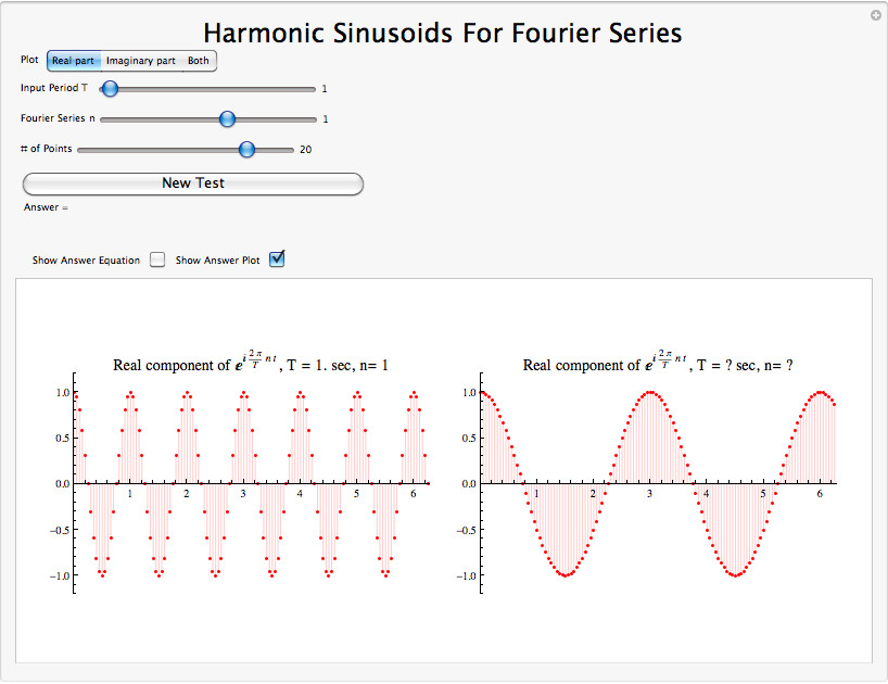
Download or Interact (when online) with a Mathematica CDF demonstrating Discrete Harmonic Sinusoids. To download, right click and save as .cdf.
DTFS Analysis
Say we have the following set of numbers that describe a periodic, discrete-time signal, where N = 4 : {…, 3, 2, -2, 1, 3, …} Such a periodic, discrete-time signal (with period N ) can be thought of as a finite set of numbers. For example, we can represent this signal as either a periodic signal or as just a single interval as follows:
Figure 7.7.
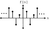
(a) Periodic Function
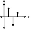
(b) Function on the interval [0, T]
Here we can look at just one period of the signal that has a vector length of four and is contained in ℂ4 .
Note
The cardinalsity of the set of discrete time signals with period N equals ℂN .
Here, we are going to form a basis using harmonic sinusoids. Before we look into this, it will be worth our time to look at the discrete-time, complex sinusoids in a little more detail.
Complex Sinusoids
If you are familiar with the basic sinusoid signal and with complex exponentials then you should not have any problem understanding this section. In most texts, you will see the the discrete-time, complex sinusoid noted as: ⅇ ⅈωn
Example 7.1.
Figure 7.8.
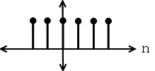
Complex sinusoid with frequency ω = 0
Example 7.2.
Figure 7.9.
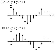
Complex sinusoid with frequency

In the Complex Plane
The complex sinusoid can be directly mapped onto our complex plane, which allows us to easily visualize changes to the complex sinusoid and extract certain properties. The absolute value of our complex sinusoid has the following characteristic: |ⅇ ⅈωn | = 1 , n ∈ ℝ which tells that our complex sinusoid only takes values on the unit circle. As for the angle, the following statement holds true: ∠ⅇ ⅈωn = wn For more information, see the section on the Discrete Time Complex Exponential to learn about Aliasing , Negative Frequencies, and the formal definition of the Complex Conjugate .
Now that we have looked over the concepts of complex sinusoids, let us turn our attention back to finding a basis for discrete-time, periodic signals. After looking at all the complex sinusoids, we must answer the question of which discrete-time sinusoids do we need to represent periodic sequences with a period N .
Equivalent Question
Find a set of vectorssuch that
are a basis for ℂ n
In answer to the above question, let us try the "harmonic" sinusoids with a fundamental frequency  :
:
(7.1)
Harmonic Sinusoid

Figure 7.10.
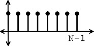
(a) Harmonic sinusoid with k = 0
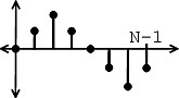
(b) Imaginary part of sinusoid,  , with k = 1
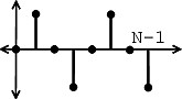
(c) Imaginary part of sinusoid,  , with k = 2
Examples of our Harmonic Sinusoids
 is periodic with period N and has k "cycles" between n = 0 and n = N − 1 .
Theorem 7.1.
If we let  where the exponential term is a vector in ℂN
, then
where the exponential term is a vector in ℂN
, then  is an orthonormal basis
for ℂN
.
is an orthonormal basis
for ℂN
.
Proof
First of all, we must show  is orthonormal, i.e. < b
k
,b
l
> = δ
kl
is orthonormal, i.e. < b
k
,b
l
> = δ
kl
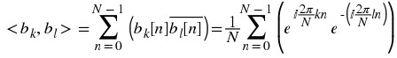
 If l = k , then
 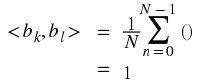 If l ≠ k , then we must use the "partial summation formula" shown below:
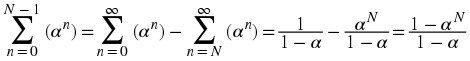
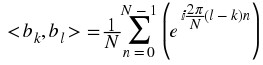 where in the above equation we can say that
 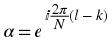 , and thus we can see how this is in the form needed to utilize our partial summation formula.
 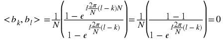 So,
So,  Therefore: {b
k
} is an orthonormal set. {b
k
} is also a basis, since there are N vectors which are linearly independent (orthogonality implies linear independence).
Therefore: {b
k
} is an orthonormal set. {b
k
} is also a basis, since there are N vectors which are linearly independent (orthogonality implies linear independence).
And finally, we have shown that the harmonic sinusoids 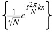 form an orthonormal basis for ℂ
n
form an orthonormal basis for ℂ
n
Periodic Extension to DTFS
Now that we have an understanding of the discrete-time Fourier series (DTFS), we can consider the periodic extension of c[k] (the Discrete-time Fourier coefficients). Figure 7.11 shows a simple illustration of how we can represent a sequence as a periodic signal mapped over an infinite number of intervals.
Figure 7.11.
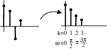
(a) vectors
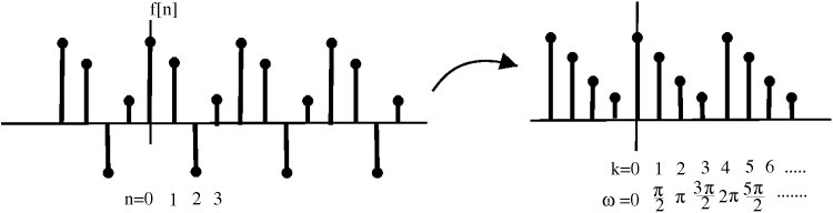
(b) periodic sequences
Exercise 7.2.1. (Go to Solution)
Why does a periodic extension to the DTFS coefficients c[k] make sense?
Examples
Example 7.3. Discrete time square wave
Figure 7.12.
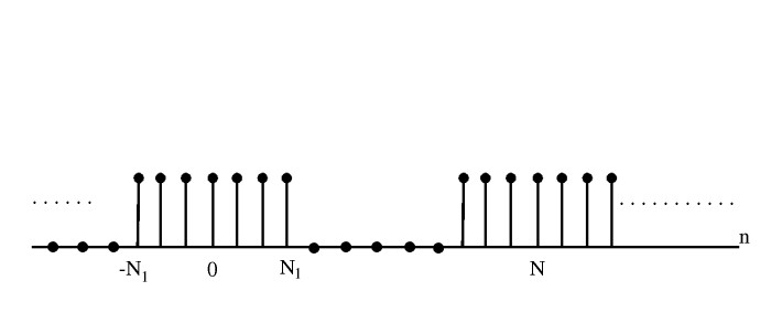
Calculate the DTFS c[k] using:Just like continuous time Fourier series, we can take the summation over any interval, so we have
Let m = n + N 1 (so we can get a geometric series starting at 0)
Now, using the "partial summation formula"
Manipulate to make this look like a sinc function (distribute):
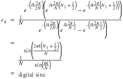
Note
It's periodic! Figure 7.13, Figure 7.14, and Figure 7.15show our above function and coefficients for various values of N 1 .
Figure 7.13.
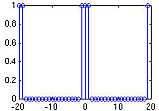
(a) Plot of f[n] .
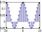
(b) Plot of c[k] .
N 1 = 1
Figure 7.14.
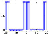
(a) Plot of f[n] .
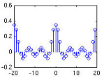
(b) Plot of c[k] .
N 1 = 3
Figure 7.15.
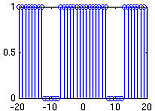
(a) Plot of f[n] .
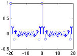
(b) Plot of c[k] .
N 1 = 7
DTFS conclusion
Using the steps shown above in the derivation and our previous understanding of Hilbert Spaces and Orthogonal Expansions, the rest of the derivation is automatic. Given a discrete-time, periodic signal (vector in ℂ
n
) f[n] , we can write: 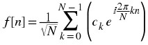
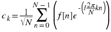 Note: Most people collect both the
  terms into the expression for c
k
.
terms into the expression for c
k
.
Discrete Time Fourier Series
Here is the common form of the DTFS with the above note taken into account: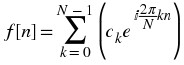
This is what the fft command in MATLAB does.
Solutions to Exercises
Solution to Exercise 7.2.1. (Return to Exercise)
Aliasing: 
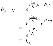 → DTFS coefficients are also periodic with period N .
7.3. Common Discrete Fourier Series*
Introduction
Once one has obtained a solid understanding of the fundamentals of Fourier series analysis and the General Derivation of the Fourier Coefficients, it is useful to have an understanding of the common signals used in Fourier Series Signal Approximation.
Deriving the Coefficients
Consider a square wave f(x) of length 1. Over the range [0,1), this can be written as 
Figure 7.16. Fourier series approximation of a square wave

Fourier series approximation to sq(t) . The number of terms in the Fourier sum is indicated in each plot, and the square wave is shown as a dashed line over two periods.
Real Even Signals
Given that the square wave is a real and even signal,
f(t) = f( – t) EVEN
f(t) = f *(t) REAL
therefore,
c n = c – n EVEN
c n = c n * REAL
Deriving the Coefficients for other signals
The Square wave is the standard example, but other important signals are also useful to analyze, and these are included here.
Constant Waveform
This signal is relatively self-explanatory: the time-varying portion of the Fourier Coefficient is taken out, and we are left simply with a constant function over all time. x ( t ) = 1
Figure 7.17. Fourier series approximation of a constant wave
Sinusoid Waveform
With this signal, only a specific frequency of time-varying Coefficient is chosen (given that the Fourier Series equation includes a sine wave, this is intuitive), and all others are filtered out, and this single time-varying coefficient will exactly match the desired signal. x ( t ) = c o s ( 2 π t )
Figure 7.18. Fourier series approximation of a sinusoid wave
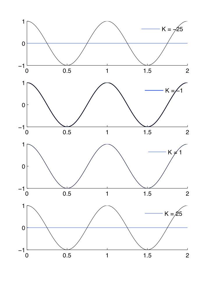
Triangle Waveform
 This is a more complex form of signal approximation to the square wave. Because of the Symmetry Properties of the Fourier Series, the triangle wave is a real and odd signal, as opposed to the real and even square wave signal. This means that
f(t) = – f( – t) ODD
f(t) = f *(t) REAL
therefore,
c n = – c – n
c n = – c n * IMAGINARY
Figure 7.19. Fourier series approximation of a triangle wave

Sawtooth Waveform
x ( t ) = t / 2 Because of the Symmetry Properties of the Fourier Series, the sawtooth wave can be defined as a real and odd signal, as opposed to the real and even square wave signal. This has important implications for the Fourier Coefficients.
Figure 7.20. Fourier series approximation of a sawtooth wave

DFT Signal Approximation
Figure 7.21.
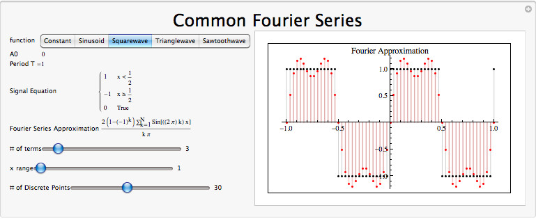
Interact (when online) with a Mathematica CDF demonstrating the common Discrete Fourier Series. To download, right-click and save as .cdf.
Conclusion
To summarize, a great deal of variety exists among the common Fourier Transforms. A summary table is provided here with the essential information.
| Description | Time Domain Signal for n ∈ Z[0,N – 1] | Frequency Domain Signal k ∈ Z[0,N – 1] |
| Constant Function | 1 | δ ( k ) |
| Unit Impulse | δ ( n ) | 
|
| Complex Exponential | e j 2 π m n / N | 
|
| Sinusoid Waveform | c o s ( j 2 π m n / N ) | 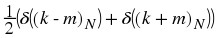
|
| Box Waveform ( M < N / 2) | 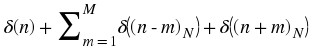
| 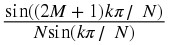
|
| Dsinc Waveform ( M < N / 2) | 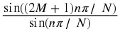
| 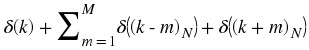
|
7.4. Properties of the DTFS*
Introduction
In this module we will discuss the basic properties of the Discrete-Time Fourier Series. We will begin by refreshing your memory of our basic Fourier series equations: 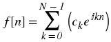
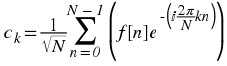 Let ℱ{·} denote the transformation from f[n] to the Fourier coefficients ℱ{f[n]} = c
k
, k ∈ ℤ ℱ{·} maps complex valued functions to sequences of complex numbers.
Let ℱ{·} denote the transformation from f[n] to the Fourier coefficients ℱ{f[n]} = c
k
, k ∈ ℤ ℱ{·} maps complex valued functions to sequences of complex numbers.
Linearity
ℱ{·} is a linear transformation.
Theorem 7.2.
If ℱ{f[n]} = c k and ℱ{g[n]} = d k . Then ℱ{α f[n]} = α c k , α ∈ ℂ and ℱ{f[n] + g[n]} = c k + d k
Proof
Easy. Just linearity of integral. 
Shifting
Shifting in time equals a phase shift of Fourier coefficients
Theorem 7.3.
ℱ{f[n − n 0]} = ⅇ – (ⅈ ω 0 k n 0) c k if c k = |c k |ⅇ ⅈ∠c k , then |ⅇ – (ⅈ ω 0 k n 0) c k | = |ⅇ – (ⅈ ω 0 k n 0)||c k | = |c k | ∠ⅇ – (ⅈ ω 0 n 0 k) = ∠c k − ω 0 n 0 k
Proof
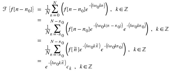
Parseval's Relation
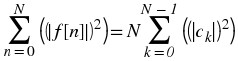 Parseval's relation tells us that the energy of a signal is equal to the energy of its Fourier transform.
Note
Parseval tells us that the Fourier series maps L 2[0, N] to l 2(ℤ) .
Figure 7.22.
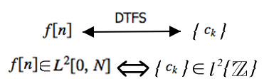
Exercise 7.4.1. (Go to Solution)
For f[n] to have "finite energy," what do the c k do as k → ∞ ?
Exercise 7.4.2. (Go to Solution)
If  , is f ∈ L
2[[0, N]] ?
, is f ∈ L
2[[0, N]] ?
Exercise 7.4.3. (Go to Solution)
Now, if  , is f ∈ L
2[[0, N]] ?
, is f ∈ L
2[[0, N]] ?
The rate of decay of the Fourier series determines if f[n] has finite energy.
ParsevalsTheorem Demonstration
Figure 7.23.
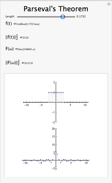
Interact (when online) with a Mathematica CDF demonstrating Parsevals Theorem. To download, right-click and save as .cdf.
Symmetry Properties
Rule 7.1. Even Signals
Even Signals
f[n] = f[ – n]
∥ c k ∥ = ∥ c – k ∥
Proof


Rule 7.2. Odd Signals
Odd Signals
f [ n ] = -f [ -n ]
c k = c – k *
Proof


Rule 7.3. Real Signals
Real Signals
f[n] = f *[n]
c k = c – k *
Proof


Differentiation in Fourier Domain
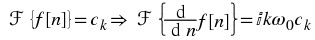
Since  then
then  A differentiator attenuates the low frequencies in f[n] and accentuates the high frequencies. It removes general trends and accentuates areas of sharp variation.
Note
A common way to mathematically measure the smoothness of a function f[n] is to see how many derivatives are finite energy.
This is done by looking at the Fourier coefficients of the signal, specifically how fast they decay as k → ∞ . If ℱ{f[n]} = c
k
and |c
k
| has the form  , then
  and has the form
  . So for the m
th derivative to have finite energy, we need
. So for the m
th derivative to have finite energy, we need 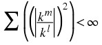 thus
thus  decays faster than
  which implies that 2l − 2m > 1 or
  Thus the decay rate of the Fourier series dictates smoothness.
Fourier Differentiation Demo
Figure 7.24.
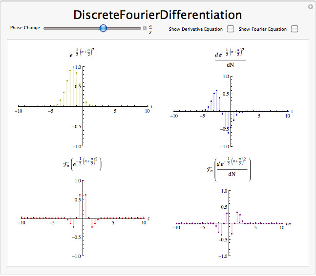
Interact (when online) with a Mathematica CDF demonstrating Differentiation in a Fourier Domain. To download, right-click and save as .cdf.
Integration in the Fourier Domain
If ℱ{f[n]} = c
k
then 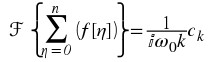
Note
If c 0 ≠ 0 , this expression doesn't make sense.
Integration accentuates low frequencies and attenuates high frequencies. Integrators bring out the general trends in signals and suppress short term variation (which is noise in many cases). Integrators are much nicer than differentiators.
Fourier Integration Demo
Figure 7.25.
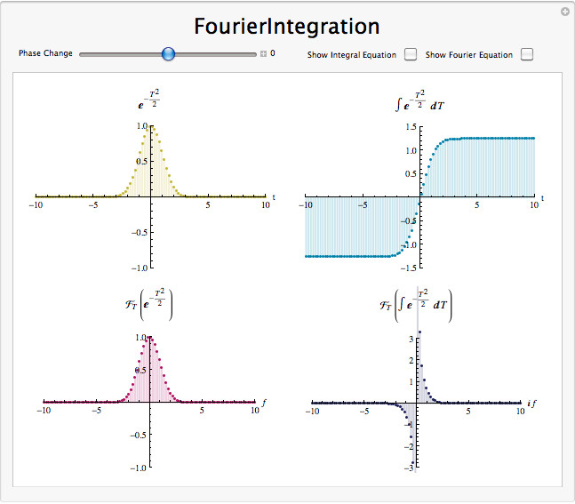
Interact (when online) with a Mathematica CDF demonstrating the effect of Integration in a Fourier Domain.To download, right-click and save as .cdf.
Signal Multiplication
Given a signal f[n] with Fourier coefficients c
k
and a signal g[n] with Fourier coefficients d
k
, we can define a new signal, y[n] , where y[n] = f[n]g[n] . We find that the Fourier Series representation of y[n] , e
k
, is such that 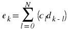 . This is to say that signal multiplication in the time domain is equivalent to discrete-time circular convolution in the frequency domain. The proof of this is as follows
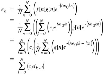
Conclusion
Like other Fourier transforms, the DTFS has many useful properties, including linearity, equal energy in the time and frequency domains, and analogs for shifting, differentation, and integration.
| Property | Signal | DTFS |
| Linearity | a x ( n ) + b y ( n ) | a X ( k ) + b Y ( k ) |
| Time Shifting | x ( n – m ) | X ( k ) e – j 2 π m k / N |
| Time Modulation | x ( n ) e j 2 π m n / N | X ( k – m ) |
| Multiplication | x ( n ) y ( n ) | X ( k ) * Y ( k ) |
| Circular Convolution | x ( n ) * y ( n ) | X ( k ) Y ( K ) |
Solutions to Exercises
Solution to Exercise 7.4.1. (Return to Exercise)
(|c k |)2 < ∞ for f[n] to have finite energy.
Solution to Exercise 7.4.2. (Return to Exercise)
Yes, because  , which is summable.
Solution to Exercise 7.4.3. (Return to Exercise)
No, because  , which is not summable.
7.5. Discrete Time Circular Convolution and the DTFS*
Introduction
This module relates circular convolution of periodic signals in one domain to multiplication in the other domain.
You should be familiar with Discrete-Time Convolution, which tells us that given two discrete-time signals x[n] , the system's input, and h[n] , the system's response, we define the output of the system as 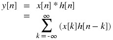 When we are given two DFTs (finite-length sequences usually of length N ), we cannot just multiply them together as we do in the above convolution formula, often referred to as linear convolution. Because the DFTs are periodic, they have nonzero values for n ≥ N and thus the multiplication of these two DFTs will be nonzero for n ≥ N . We need to define a new type of convolution operation that will result in our convolved signal being zero outside of the range n = {0, 1, …, N − 1} . This idea led to the development of circular convolution, also called cyclic or periodic convolution.
Signal Circular Convolution
Given a signal f[n] with Fourier coefficients c
k
and a signal g[n] with Fourier coefficients d
k
, we can define a new signal, v[n] , where v[n] = (f[n] ⊛ g[n]) We find that the Fourier Series representation of v[n] , a
k
, is such that a
k
= c
k
d
k
. (f[n] ⊛ g[n]) is the circular convolution of two periodic signals and is equivalent to the convolution over one interval, i.e.
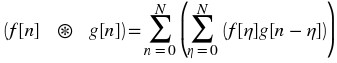 .
.
Note
Circular convolution in the time domain is equivalent to multiplication of the Fourier coefficients.
This is proved as follows 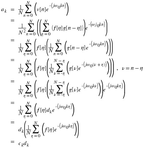
Circular Convolution Formula
What happens when we multiply two DFT's together, where Y[k] is the DFT of y[n] ? Y[k] = F[k]H[k] when 0 ≤ k ≤ N − 1
Using the DFT synthesis formula for y[n] 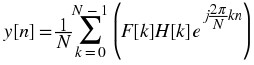
And then applying the analysis formula 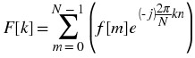
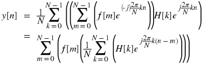 where we can reduce the second summation found in the above equation into
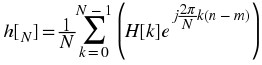
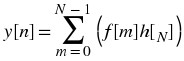 which equals circular convolution! When we have 0 ≤ n ≤ N − 1 in the above, then we get: y[n] ≡ (f[n] ⊛ h[n])
Note
The notation ⊛ represents cyclic convolution "mod N".
Alternative Convolution Formula
Alternative Circular Convolution Algorithm
Step 1: Calculate the DFT of f[n] which yields F[k] and calculate the DFT of h[n] which yields H[k] .
Step 2: Pointwise multiply Y[k] = F[k]H[k]
Step 3: Inverse DFT Y[k] which yields y[n]
Seems like a roundabout way of doing things, but it turns out that there are extremely fast ways to calculate the DFT of a sequence.
To circularily convolve 2 N -point sequences:  For each n : N multiples, N − 1 additions
N points implies N 2 multiplications, N(N − 1) additions implies O(N 2) complexity.
Steps for Circular Convolution
We can picture periodic sequences as having discrete points on a circle as the domain
Figure 7.26.
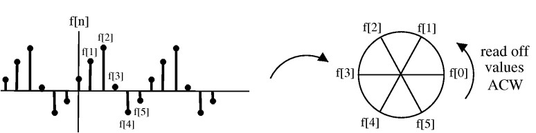
Shifting by m , f(n + m) , corresponds to rotating the cylinder m notches ACW (counter clockwise). For m = -2 , we get a shift equal to that in the following illustration:
Figure 7.27.

for m = -2
Figure 7.28.
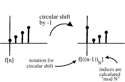
To cyclic shift we follow these steps:
1) Write f(n) on a cylinder, ACW
Figure 7.29.

N = 8
2) To cyclic shift by m , spin cylinder m spots ACW (f[n] → f[ (( n + m )) N ])
Figure 7.30.
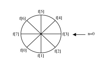
m = -3
Notes on circular shifting
f[ (( n + N )) N ] = f[n] Spinning N spots is the same as spinning all the way around, or not spinning at all.
f[ (( n + N )) N ] = f[ (( n – ( N – m ) )) N ] Shifting ACW m is equivalent to shifting CW N − m
Figure 7.31.
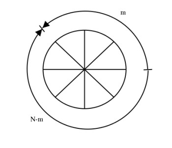
f[ (( – n )) N ] The above expression, simply writes the values of f[n] clockwise.
Figure 7.32.
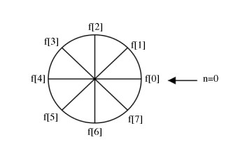
(a) f[n]
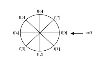
(b) f[ (( – n )) N ]
Example 7.4. Convolve (n = 4)
Figure 7.33.
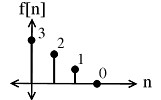
(a)
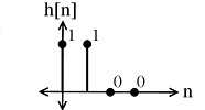
(b)
Two discrete-time signals to be convolved.

Figure 7.34.
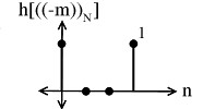
Multiply f[m] and sum to yield: y[0] = 3

Figure 7.35.
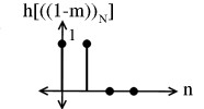
Multiply f[m] and sum to yield: y[1] = 5

Figure 7.36.
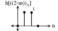
Multiply f[m] and sum to yield: y[2] = 3

Figure 7.37.
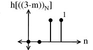
Multiply f[m] and sum to yield: y[3] = 1
Exercise
Take a look at a square pulse with a period of T.
For this signal 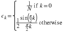
Take a look at a triangle pulse train with a period of T.
This signal is created by circularly convolving the square pulse with itself. The Fourier coefficients for this signal are 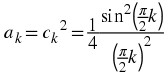
Exercise 7.5.1. (Go to Solution)
Find the Fourier coefficients of the signal that is created when the square pulse and the triangle pulse are convolved.
Circular Shifts and the DFT
Theorem 7.4. Circular Shifts and DFT
If  then
then  (i.e. circular shift in time domain = phase shift in DFT)
Proof
 so phase shifting the DFT
Circular Convolution Demonstration
Figure 7.38.
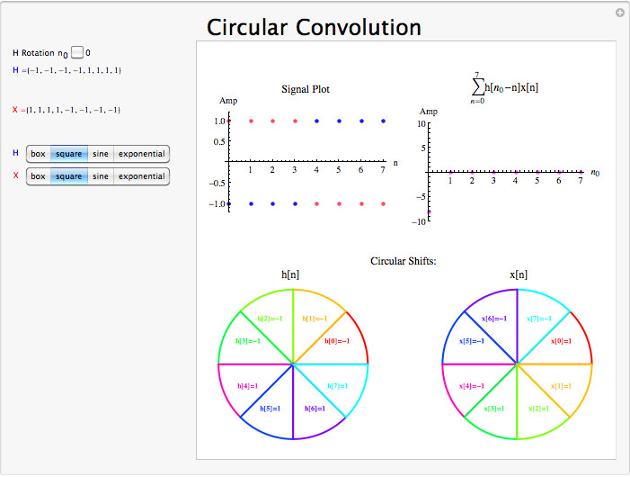
Interact (when online) with a Mathematica CDF demonstrating Circular Shifts.
Conclusion
Circular convolution in the time domain is equivalent to multiplication of the Fourier coefficients in the frequency domain.
Solutions to Exercises
Solution to Exercise 7.5.1. (Return to Exercise)
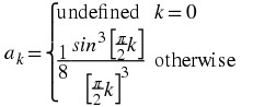
Chapter 8. Continuous Time Fourier Transform (CTFT)
8.1. Continuous Time Aperiodic Signals*
Introduction
This module describes the type of signals acted on by the Continuous Time Fourier Transform.
Relevant Spaces
The Continuous-Time Fourier Transform maps infinite-length (a-periodic), continuous-time signals in L 2 to infinite-length, discrete-frequency signals in l 2 .
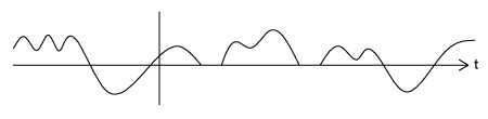
Periodic and Aperiodic Signals
When a function repeats itself exactly after some given period, or cycle, we say it's periodic. A periodic function can be mathematically defined as: f(t) = f(t + mT) m ∈ ℤ where T > 0 represents the fundamental period of the signal, which is the smallest positive value of T for the signal to repeat. Because of this, you may also see a signal referred to as a T-periodic signal. Any function that satisfies this equation is said to be periodic with period T.
An aperiodic CT function f(t) does not repeat for any T ∈ ℝ ; i.e. there exists no T such that this equation holds.
Suppose we have such an aperiodic function f(t) . We can construct a periodic extension of f(t) called f To(t) , where f(t) is repeated every T 0 seconds. If we take the limit as T 0 → ∞ , we obtain a precise model of an aperiodic signal for which all rules that govern periodic signals can be applied, including Fourier Analysis (with an important modification). For more detail on this distinction, see the module on the Continuous Time Fourier Transform.
Aperiodic Signal Demonstration
Figure 8.1.
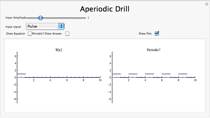
Interact (when online) with a Mathematica CDF demonstrating Periodic versus Aperiodic Signals.To download, right-click and save as .cdf.
Conclusion
Any aperiodic signal can be defined by an infinite sum of periodic functions, a useful definition that makes it possible to use Fourier Analysis on it by assuming all frequencies are present in the signal.
8.2. Continuous Time Fourier Transform (CTFT)*
Introduction
In this module, we will derive an expansion for any arbitrary continuous-time function, and in doing so, derive the Continuous Time Fourier Transform (CTFT).
Since complex exponentials are eigenfunctions of linear time-invariant (LTI) systems, calculating the output of an LTI system ℋ given ⅇ st as an input amounts to simple multiplication, where H(s) ∈ ℂ is the eigenvalue corresponding to s. As shown in the figure, a simple exponential input would yield the output y(t) = H(s)ⅇ st

Using this and the fact that ℋ is linear, calculating y(t) for combinations of complex exponentials is also straightforward.
c
1
ⅇ
s
1
t
+ c
2
ⅇ
s
2
t
→ c
1
H(s
1)ⅇ
s
1
t
+ c
2
H(s
2)ⅇ
s
2
t

The action of H on an input such as those in the two equations above is easy to explain. ℋ independently scales each exponential component ⅇ s n t by a different complex number H(s n ) ∈ ℂ . As such, if we can write a function f(t) as a combination of complex exponentials it allows us to easily calculate the output of a system.
Now, we will look to use the power of complex exponentials to see how we may represent arbitrary signals in terms of a set of simpler functions by superposition of a number of complex exponentials. Below we will present the Continuous-Time Fourier Transform (CTFT), commonly referred to as just the Fourier Transform (FT). Because the CTFT deals with nonperiodic signals, we must find a way to include all real frequencies in the general equations. For the CTFT we simply utilize integration over real numbers rather than summation over integers in order to express the aperiodic signals.
Fourier Transform Synthesis
Joseph Fourier demonstrated that an arbitrary s(t) can be written as a linear combination of harmonic complex sinusoids 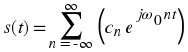 where
where  is the fundamental frequency. For almost all s(t) of practical interest, there exists c
n
to make Equation true. If s(t) is finite energy ( s(t) ∈ L
2[0, T] ), then the equality in Equation holds in the sense of energy convergence; if s(t) is continuous, then Equation holds pointwise. Also, if s(t) meets some mild conditions (the Dirichlet conditions), then Equation holds pointwise everywhere except at points of discontinuity.
is the fundamental frequency. For almost all s(t) of practical interest, there exists c
n
to make Equation true. If s(t) is finite energy ( s(t) ∈ L
2[0, T] ), then the equality in Equation holds in the sense of energy convergence; if s(t) is continuous, then Equation holds pointwise. Also, if s(t) meets some mild conditions (the Dirichlet conditions), then Equation holds pointwise everywhere except at points of discontinuity.
The c n - called the Fourier coefficients - tell us "how much" of the sinusoid ⅇ j ω 0 n t is in s(t) . The formula shows s(t) as a sum of complex exponentials, each of which is easily processed by an LTI system (since it is an eigenfunction of every LTI system). Mathematically, it tells us that the set of complex exponentials {ⅇ j ω 0 n t , n ∈ ℤ } form a basis for the space of T-periodic continuous time functions.
Equations
Now, in order to take this useful tool and apply it to arbitrary non-periodic signals, we will have to delve deeper into the use of the superposition principle. Let s
T
(t) be a periodic signal having period T . We want to consider what happens to this signal's spectrum as the period goes to infinity. We denote the spectrum for any assumed value of the period by c
n
(T). We calculate the spectrum according to the Fourier formula for a periodic signal, known as the Fourier Series (for more on this derivation, see the section on Fourier Series.)  where
where  and where we have used a symmetric placement of the integration interval about the origin for subsequent derivational convenience. We vary the frequency index n proportionally as we increase the period. Define
  making the corresponding Fourier Series
 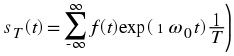 As the period increases, the spectral lines become closer together, becoming a continuum. Therefore,
 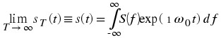 with
with 
(8.1)
Continuous-Time Fourier Transform

(8.2)
Inverse CTFT

Warning
It is not uncommon to see the above formula written slightly different. One of the most common differences is the way that the exponential is written. The above equations use the radial frequency variable Ω in the exponential, where Ω = 2π f , but it is also common to include the more explicit expression, ⅈ2πft , in the exponential. Click here for an overview of the notation used in Connexion's DSP modules.
Example 8.1.
We know from Euler's formula that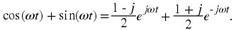
CTFT Definition Demonstration
Figure 8.2.
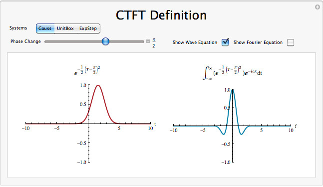
Interact (when online) with a Mathematica CDF demonstrating Continuous Time Fourier Transform. To Download, right-click and save as .cdf.
Example Problems
Exercise 8.2.1. (Go to Solution)
Find the Fourier Transform (CTFT) of the function 
Exercise 8.2.2. (Go to Solution)
Find the inverse Fourier transform of the ideal lowpass filter defined by 
Fourier Transform Summary
Because complex exponentials are eigenfunctions of LTI systems, it is often useful to represent signals using a set of complex exponentials as a basis. The continuous time Fourier series synthesis formula expresses a continuous time, periodic function as the sum of continuous time, discrete frequency complex exponentials.  The continuous time Fourier series analysis formula gives the coefficients of the Fourier series expansion.
  In both of these equations
  is the fundamental frequency.
Solutions to Exercises
Solution to Exercise 8.2.1. (Return to Exercise)
In order to calculate the Fourier transform, all we need to use is Equation 8.1, complex exponentials, and basic calculus. 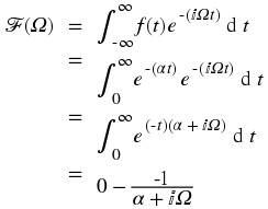
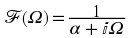
Solution to Exercise 8.2.2. (Return to Exercise)
Here we will use Equation 8.2 to find the inverse FT given that t ≠ 0 . 
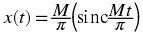
8.3. Common Fourier Transforms*
Common CTFT Properties
| Time Domain Signal | Frequency Domain Signal | Condition |
|---|---|---|
| ⅇ – (at) u(t) | 
| a > 0 |
| ⅇ at u( – t) | 
| a > 0 |
| ⅇ – (a|t|) | 
| a > 0 |
| t ⅇ – (at) u(t) | 
| a > 0 |
| t n ⅇ – (at) u(t) | 
| a > 0 |
| δ(t) | 1 | |
| 1 | 2 π δ(ω) | |
| ⅇ ⅈ ω 0 t | 2 π δ(ω − ω 0) | |
| cos( ω 0 t) | π(δ(ω − ω 0) + δ(ω + ω 0)) | |
| sin( ω 0 t) | ⅈ π(δ(ω + ω 0) − δ(ω − ω 0)) | |
| u(t) | 
| |
| sgn( t) | 
| |
| cos( ω 0 t)u(t) | 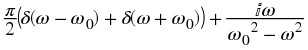
| |
| sin( ω 0 t)u(t) | 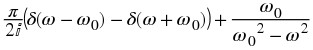
| |
| ⅇ – (at)sin(ω 0 t)u(t) | 
| a > 0 |
| ⅇ – (at)cos(ω 0 t)u(t) | 
| a > 0 |
| u(t + τ) − u(t − τ) | 
| |
| u(ω + ω 0) − u(ω − ω 0) | |

| 
| |
| 
| |
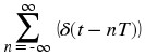
| 
| 
|

| 
|
triag[n] is the triangle function for arbitrary real-valued n .
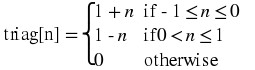
8.4. Properties of the CTFT*
Introduction
This module will look at some of the basic properties of the Continuous-Time Fourier Transform (CTFT).
Note
We will be discussing these properties for aperiodic, continuous-time signals but understand that very similar properties hold for discrete-time signals and periodic signals as well.
Discussion of Fourier Transform Properties
Linearity
The combined addition and scalar multiplication properties in the table above demonstrate the basic property of linearity. What you should see is that if one takes the Fourier transform of a linear combination of signals then it will be the same as the linear combination of the Fourier transforms of each of the individual signals. This is crucial when using a table of transforms to find the transform of a more complicated signal.
Example 8.2.
We will begin with the following signal: z(t) = a f 1(t) + b f 2(t) Now, after we take the Fourier transform, shown in the equation below, notice that the linear combination of the terms is unaffected by the transform. Z(ω) = a F 1(ω) + b F 2(ω)
Symmetry
Symmetry is a property that can make life quite easy when solving problems involving Fourier transforms. Basically what this property says is that since a rectangular function in time is a sinc function in frequency, then a sinc function in time will be a rectangular function in frequency. This is a direct result of the similarity between the forward CTFT and the inverse CTFT. The only difference is the scaling by 2π and a frequency reversal.
Time Scaling
This property deals with the effect on the frequency-domain representation of a signal if the time variable is altered. The most important concept to understand for the time scaling property is that signals that are narrow in time will be broad in frequency and vice versa. The simplest example of this is a delta function, a unit pulse with a very small duration, in time that becomes an infinite-length constant function in frequency.
The table above shows this idea for the general transformation from the time-domain to the frequency-domain of a signal. You should be able to easily notice that these equations show the relationship mentioned previously: if the time variable is increased then the frequency range will be decreased.
Time Shifting
Time shifting shows that a shift in time is equivalent to a linear phase shift in frequency. Since the frequency content depends only on the shape of a signal, which is unchanged in a time shift, then only the phase spectrum will be altered. This property is proven below:
Example 8.3.
We will begin by letting z(t) = f(t − τ) . Now let us take the Fourier transform with the previous expression substituted in for z(t) .Now let us make a simple change of variables, where σ = t − τ . Through the calculations below, you can see that only the variable in the exponential are altered thus only changing the phase in the frequency domain.
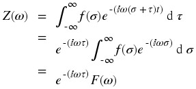
Convolution
Convolution is one of the big reasons for converting signals to the frequency domain, since convolution in time becomes multiplication in frequency. This property is also another excellent example of symmetry between time and frequency. It also shows that there may be little to gain by changing to the frequency domain when multiplication in time is involved.
We will introduce the convolution integral here, but if you have not seen this before or need to refresh your memory, then look at the continuous-time convolution module for a more in depth explanation and derivation.
(8.3)
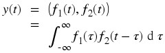
Time Differentiation
Since LTI systems can be represented in terms of differential equations, it is apparent with this property that converting to the frequency domain may allow us to convert these complicated differential equations to simpler equations involving multiplication and addition. This is often looked at in more detail during the study of the Laplace Transform.
Parseval's Relation
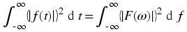 Parseval's relation tells us that the energy of a signal is equal to the energy of its Fourier transform.
Figure 8.3.
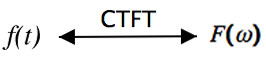
Modulation (Frequency Shift)
Modulation is absolutely imperative to communications applications. Being able to shift a signal to a different frequency, allows us to take advantage of different parts of the electromagnetic spectrum is what allows us to transmit television, radio and other applications through the same space without significant interference.
The proof of the frequency shift property is very similar to that of the time shift; however, here we would use the inverse Fourier transform in place of the Fourier transform. Since we went through the steps in the previous, time-shift proof, below we will just show the initial and final step to this proof: 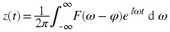 Now we would simply reduce this equation through another change of variables and simplify the terms. Then we will prove the property expressed in the table above: z(t) = f(t)ⅇ
ⅈφt
Now we would simply reduce this equation through another change of variables and simplify the terms. Then we will prove the property expressed in the table above: z(t) = f(t)ⅇ
ⅈφt
Properties Demonstration
An interactive example demonstration of the properties is included below:
Figure 8.4.
(This media type is not supported in this reader. Click to open media in browser.)
Interactive Signal Processing Laboratory Virtual Instrument created using NI's Labview.
Summary Table of CTFT Properties
| Operation Name | Signal ( f(t) ) | Transform ( F(ω) ) |
|---|---|---|
| Linearity | a(f 1, t) + b(f 2, t) | a(F 1, ω) + b(F 2, ω) |
| Scalar Multiplication | α f(t) | α F(ω) |
| Symmetry | F(t) | 2 π f( – ω) |
| Time Scaling | f(αt) | 
|
| Time Shift | f(t − τ) | F(ω)ⅇ – (ⅈωτ) |
| Convolution in Time | ( f 1(t), f 2(t)) | F 1(t)F 2(t) |
| Convolution in Frequency | f 1(t)f 2(t) | 
|
| Differentiation | 
| ( ⅈω)n F(ω) |
| Parseval's Theorem | 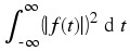
| 
|
| Modulation (Frequency Shift) | f(t)ⅇ ⅈφt | F(ω − φ) |
8.5. Continuous Time Convolution and the CTFT*
Introduction
This module discusses convolution of continuous signals in the time and frequency domains.
Continuous Time Fourier Transform
The CTFT transforms a infinite-length continuous signal in the time domain into an infinite-length continuous signal in the frequency domain.
(8.4)
CTFT

(8.5)
Inverse CTFT

Convolution Integral
The convolution integral expresses the output of an LTI system based on an input signal, x(t) , and the system's impulse response, h(t) . The convolution integral is expressed as 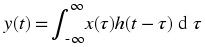 Convolution is such an important tool that it is represented by the symbol * , and can be written as y(t) = x(t) * h(t) Convolution is commutative. For more information on the characteristics of the convolution integral, read about the Properties of Convolution.
Demonstration
Figure 8.5.
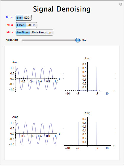
Interact (when online) with a Mathematica CDF demonstrating Use of the CTFT in signal denoising. To Download, right-click and save target as .cdf.
Convolution Theorem
Let f and g be two functions with convolution f * g .. Let F be the Fourier transform operator. Then
(8.6)F ( f * g ) = F ( f ) · F ( g )
(8.7)F ( f · g ) = F ( f ) * F ( g )
By applying the inverse Fourier transform F – 1 , we can write:
(8.8)f * g = F – 1 ( F ( f ) · F ( g ) )
Conclusion
The Fourier transform of a convolution is the pointwise product of Fourier transforms. In other words, convolution in one domain (e.g., time domain) corresponds to point-wise multiplication in the other domain (e.g., frequency domain).
Chapter 9. Discrete Time Fourier Transform (DTFT)
9.1. Discrete Time Aperiodic Signals*
Introduction
This module describes the type of signals acted on by the Discrete Time Fourier Transform.
Relevant Spaces
The Discrete Time Fourier Transform maps arbitrary discrete time signals in l 2(ℤ) to finite-length, discrete-frequency signals in L 2([0, 2π)) .
Figure 9.1.
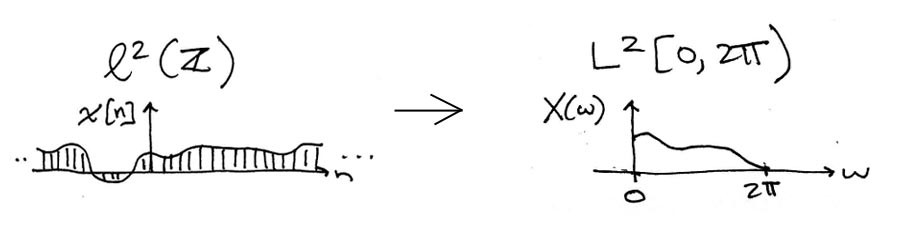
Mapping l 2(ℤ) in the time domain to L 2([0, 2π)) in the frequency domain.
Periodic and Aperiodic Signals
When a function repeats itself exactly after some given period, or cycle, we say it's periodic. A periodic function can be mathematically defined as: f[n] = f[n + mN] m ∈ ℤ where N > 0 represents the fundamental period of the signal, which is the smallest positive value of N for the signal to repeat. Because of this, you may also see a signal referred to as an N-periodic signal. Any function that satisfies this equation is said to be periodic with period N. Periodic signals in discrete time repeats themselves in each cycle. However, only integers are allowed as time variable in discrete time. We denote signals in such case as f[n], n = ..., -2, -1, 0, 1, 2, ... Here's an example of a discrete-time periodic signal with period N:
Figure 9.2. discrete-time periodic signal
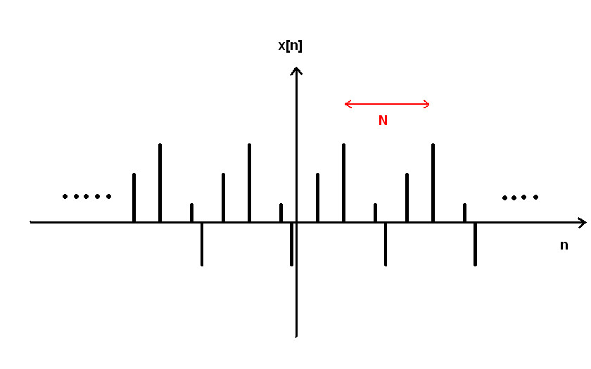
Notice the function is the same after a time shift of N
We can think of periodic functions (with period N ) two different ways:
as functions on all of ℝ
Figure 9.3.
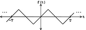
discrete time periodic function over all of ℝ where f[n 0] = f[n 0 + N]
or, we can cut out all of the redundancy, and think of them as functions on an interval
 (or, more generally,
  ). If we know the signal is N-periodic then all the information of the signal is captured by the above interval.
 Figure 9.4.

Remove the redundancy of the period function so that f[n] is undefined outside
 .
.
An aperiodic DT function, however, f[n] does not repeat for any N ∈ ℝ ; i.e. there exists no N such that this equation holds. This broader class of signals can only be acted upon by the DTFT.
Suppose we have such an aperiodic function f[n] . We can construct a periodic extension of f[n] called f No[n] , where f[n] is repeated every N 0 seconds. If we take the limit as N 0 → ∞ , we obtain a precise model of an aperiodic signal for which all rules that govern periodic signals can be applied, including Fourier Analysis (with an important modification). For more detail on this distinction, see the module on the Discete Time Fourier Transform.
Aperiodic Signal Demonstration
Figure 9.5.
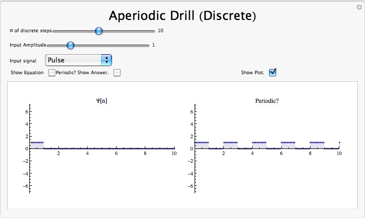
Click on the above thumbnail image (when online) to download an interactive Mathematica Player testing Periodic versus Aperiodic Signals. To download, right-click and save as .cdf.
Conclusion
A discrete periodic signal is completely defined by its values in one period, such as the interval [0,N]. Any aperiodic signal can be defined as an infinite sum of periodic functions, a useful definition that makes it possible to use Fourier Analysis on it by assuming all frequencies are present in the signal.
9.2. Discrete Time Fourier Transform (DTFT)*
Introduction
In this module, we will derive an expansion for arbitrary discrete-time functions, and in doing so, derive the Discrete Time Fourier Transform (DTFT).
Since complex exponentials are eigenfunctions of linear time-invariant (LTI) systems, calculating the output of an LTI system ℋ given ⅇ
ⅈωn
as an input amounts to simple multiplication, where  , and where H[k] ∈ ℂ is the eigenvalue corresponding to k. As shown in the figure, a simple exponential input would yield the output y[n] = H[k]ⅇ
ⅈωn
, and where H[k] ∈ ℂ is the eigenvalue corresponding to k. As shown in the figure, a simple exponential input would yield the output y[n] = H[k]ⅇ
ⅈωn
Figure 9.6.

Simple LTI system.
Using this and the fact that ℋ is linear, calculating y[n] for combinations of complex exponentials is also straightforward.
c
1
ⅇ
ⅈ
ω
1
n
+ c
2
ⅇ
ⅈ
ω
2
n
→ c
1
H[k
1]ⅇ
ⅈ
ω
1
n
+ c
2
H[k
2]ⅇ
ⅈ
ω
1
n

The action of H on an input such as those in the two equations above is easy to explain. ℋ independently scales each exponential component ⅇ ⅈ ω l n by a different complex number H[k l ] ∈ ℂ . As such, if we can write a function y[n] as a combination of complex exponentials it allows us to easily calculate the output of a system.
Now, we will look to use the power of complex exponentials to see how we may represent arbitrary signals in terms of a set of simpler functions by superposition of a number of complex exponentials. Below we will present the Discrete-Time Fourier Transform (DTFT). Because the DTFT deals with nonperiodic signals, we must find a way to include all real frequencies in the general equations. For the DTFT we simply utilize summation over all real numbers rather than summation over integers in order to express the aperiodic signals.
DTFT synthesis
It can be demonstrated that an arbitrary Discrete Time-periodic function
f[n] can be written as a linear combination of harmonic complex sinusoids 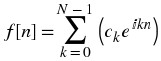 where
where  is the fundamental frequency. For almost all f[n] of practical interest, there exists c
n
to make Equation true. If f[n] is finite energy ( f[n] ∈ L
2[0, N] ), then the equality in Equation holds in the sense of energy convergence; with discrete-time signals, there are no concerns for divergence as there are with continuous-time signals.
is the fundamental frequency. For almost all f[n] of practical interest, there exists c
n
to make Equation true. If f[n] is finite energy ( f[n] ∈ L
2[0, N] ), then the equality in Equation holds in the sense of energy convergence; with discrete-time signals, there are no concerns for divergence as there are with continuous-time signals.
The c n - called the Fourier coefficients - tell us "how much" of the sinusoid ⅇ j ω 0 k n is in f[n] . The formula shows f[n] as a sum of complex exponentials, each of which is easily processed by an LTI system (since it is an eigenfunction of every LTI system). Mathematically, it tells us that the set of complex exponentials {ⅇ j ω 0 k n , k ∈ ℤ } form a basis for the space of N-periodic discrete time functions.
Equations
Now, in order to take this useful tool and apply it to arbitrary non-periodic signals, we will have to delve deeper into the use of the superposition principle. Let s
T
(t) be a periodic signal having period T . We want to consider what happens to this signal's spectrum as the period goes to infinity. We denote the spectrum for any assumed value of the period by c
n
(T). We calculate the spectrum according to the Fourier formula for a periodic signal, known as the Fourier Series (for more on this derivation, see the section on Fourier Series.) 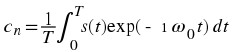 where
where  and where we have used a symmetric placement of the integration interval about the origin for subsequent derivational convenience. We vary the frequency index n proportionally as we increase the period. Define
 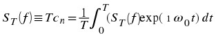 making the corresponding Fourier Series
  As the period increases, the spectral lines become closer together, becoming a continuum. Therefore,
  with
with 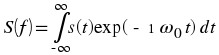
(9.1)
Discrete-Time Fourier Transform

(9.2)
Inverse DTFT

Warning
It is not uncommon to see the above formula written slightly different. One of the most common differences is the way that the exponential is written. The above equations use the radial frequency variable ω in the exponential, where ω = 2π f , but it is also common to include the more explicit expression, ⅈ2πft , in the exponential. Sometimes DTFT notation is expressed as F(ⅇ ⅈω ) , to make it clear that it is not a CTFT (which is denoted as F(Ω) ). Click here for an overview of the notation used in Connexion's DSP modules.
DTFT Definition demonstration
Figure 9.7.
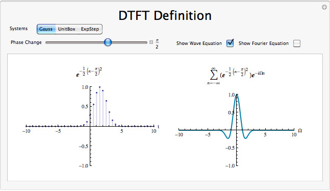
Click on the above thumbnail image (when online) to download an interactive Mathematica Player demonstrating Discrete Time Fourier Transform. To Download, right-click and save target as .cdf.
DTFT Summary
Because complex exponentials are eigenfunctions of LTI systems, it is often useful to represent signals using a set of complex exponentials as a basis. The discrete time Fourier transform synthesis formula expresses a discrete time, aperiodic function as the infinite sum of continuous frequency complex exponentials. 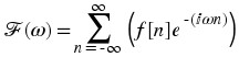 The discrete time Fourier transform analysis formula takes the same discrete time domain signal and represents the signal in the continuous frequency domain.
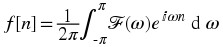
9.3. Common Discrete Time Fourier Transforms*
Common DTFTs
| Time Domain x[n] | Frequency Domain X(w) | Notes |
| δ [ n ] | 1 | |
| δ[n – M] | e – j w M | integer M |
| ∑ ∞ m = – ∞ δ[n – M m] | 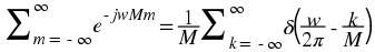
| integer M |
| e – j a n | 2 π δ ( w + a ) | real number a |
| u[n] | 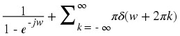
| |
| a n u(n) | 
| if | a| < 1 |
| c o s(a n) | π [ δ ( w – a ) + δ ( w + a ) ] | real number a |
| s i n c[(a + n)] | e jaw | real number a |
| W · s i n c 2(W n) | 
| real number W, 0 < W ≤ 0 . 5 |
| W · s i n c[W(n + a)] | 
| real numbers W,a 0 < W ≤ 1 |
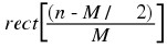
| 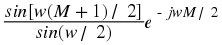
| integer M |
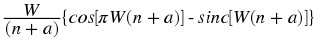
| 
| real numbers W,a 0 < W ≤ 1 |
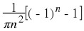
| | w | | |
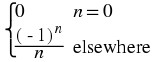
| jw | differentiator filter |
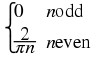
| 
| Hilbert Transform |
Notes
rect(t) is the rectangle function for arbitrary real-valued t .
(9.3)
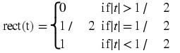
tri(t) is the triangle function for arbitrary real-valued t .
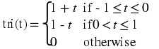
9.4. Properties of the DTFT*
Introduction
This module will look at some of the basic properties of the Discrete-Time Fourier Transform (DTFT).
Note
We will be discussing these properties for aperiodic, discrete-time signals but understand that very similar properties hold for continuous-time signals and periodic signals as well.
Discussion of Fourier Transform Properties
Linearity
The combined addition and scalar multiplication properties in the table above demonstrate the basic property of linearity. What you should see is that if one takes the Fourier transform of a linear combination of signals then it will be the same as the linear combination of the Fourier transforms of each of the individual signals. This is crucial when using a table of transforms to find the transform of a more complicated signal.
Example 9.1.
We will begin with the following signal: z[n] = a f 1[n] + b f 2[n] Now, after we take the Fourier transform, shown in the equation below, notice that the linear combination of the terms is unaffected by the transform. Z(ω) = a F 1(ω) + b F 2(ω)
Symmetry
Symmetry is a property that can make life quite easy when solving problems involving Fourier transforms. Basically what this property says is that since a rectangular function in time is a sinc function in frequency, then a sinc function in time will be a rectangular function in frequency. This is a direct result of the similarity between the forward DTFT and the inverse DTFT. The only difference is the scaling by 2π and a frequency reversal.
Time Scaling
This property deals with the effect on the frequency-domain representation of a signal if the time variable is altered. The most important concept to understand for the time scaling property is that signals that are narrow in time will be broad in frequency and vice versa. The simplest example of this is a delta function, a unit pulse with a very small duration, in time that becomes an infinite-length constant function in frequency.
The table above shows this idea for the general transformation from the time-domain to the frequency-domain of a signal. You should be able to easily notice that these equations show the relationship mentioned previously: if the time variable is increased then the frequency range will be decreased.
Time Shifting
Time shifting shows that a shift in time is equivalent to a linear phase shift in frequency. Since the frequency content depends only on the shape of a signal, which is unchanged in a time shift, then only the phase spectrum will be altered. This property is proven below:
Example 9.2.
We will begin by letting z[n] = f[n − η] . Now let us take the Fourier transform with the previous expression substituted in for z[n] .Now let us make a simple change of variables, where σ = n − η . Through the calculations below, you can see that only the variable in the exponential are altered thus only changing the phase in the frequency domain.
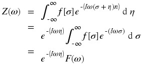
Convolution
Convolution is one of the big reasons for converting signals to the frequency domain, since convolution in time becomes multiplication in frequency. This property is also another excellent example of symmetry between time and frequency. It also shows that there may be little to gain by changing to the frequency domain when multiplication in time is involved.
We will introduce the convolution integral here, but if you have not seen this before or need to refresh your memory, then look at the discrete-time convolution module for a more in depth explanation and derivation.
(9.4)
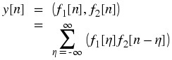
Time Differentiation
Since LTI systems can be represented in terms of differential equations, it is apparent with this property that converting to the frequency domain may allow us to convert these complicated differential equations to simpler equations involving multiplication and addition. This is often looked at in more detail during the study of the Z Transform.
Parseval's Relation
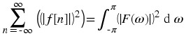 Parseval's relation tells us that the energy of a signal is equal to the energy of its Fourier transform.
Figure 9.8.
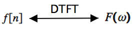
Modulation (Frequency Shift)
Modulation is absolutely imperative to communications applications. Being able to shift a signal to a different frequency, allows us to take advantage of different parts of the electromagnetic spectrum is what allows us to transmit television, radio and other applications through the same space without significant interference.
The proof of the frequency shift property is very similar to that of the time shift; however, here we would use the inverse Fourier transform in place of the Fourier transform. Since we went through the steps in the previous, time-shift proof, below we will just show the initial and final step to this proof:  Now we would simply reduce this equation through another change of variables and simplify the terms. Then we will prove the property expressed in the table above: z(t) = f(t)ⅇ
ⅈφt
Now we would simply reduce this equation through another change of variables and simplify the terms. Then we will prove the property expressed in the table above: z(t) = f(t)ⅇ
ⅈφt
Properties Demonstration
An interactive example demonstration of the properties is included below:
Figure 9.9.
(This media type is not supported in this reader. Click to open media in browser.)
Interactive Signal Processing Laboratory Virtual Instrument created using NI's Labview.
Summary Table of DTFT Properties
| Sequence Domain | Frequency Domain | |
|---|---|---|
| Linearity | a 1 s 1(n) + a2 s 2(n) | a 1 S 1(ⅇ ⅈ2π f ) + a2 S 2(ⅇ ⅈ2π f ) |
| Conjugate Symmetry | s(n) real | 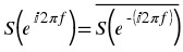
|
| Even Symmetry | s(n) = s( – n) | S(ⅇ ⅈ2π f ) = S(ⅇ – (ⅈ2π f)) |
| Odd Symmetry | s(n) = – (s( – n)) | S(ⅇ ⅈ2π f ) = – (S(ⅇ – (ⅈ2π f))) |
| Time Delay | s(n − n 0 ) | ⅇ – (ⅈ2π f n 0 ) S(ⅇ ⅈ2π f ) |
| Multiplication by n | n s(n) | 
|
| Sum | 
| S(ⅇ ⅈ2π0) |
| Value at Origin | s(0) | 
|
| Parseval's Theorem | 
| 
|
| Complex Modulation | ⅇ ⅈ2π f 0 n s(n) | S(ⅇ ⅈ2π(f − f 0 )) |
| Amplitude Modulation | s(n)cos(2π f 0 n) | 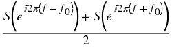
|
| s(n)sin(2π f 0 n) | 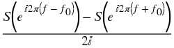
|
9.5. Discrete Time Convolution and the DTFT*
Introduction
This module discusses convolution of discrete signals in the time and frequency domains.
The Discrete-Time Convolution
Discrete Time Fourier Transform
The DTFT transforms an infinite-length discrete signal in the time domain into an finite-length (or 2π -periodic) continuous signal in the frequency domain.
(9.5)
DTFT
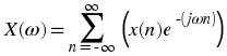
(9.6)
Inverse DTFT
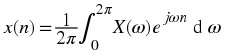
Demonstration
Figure 9.10.

Interact (when online) with a Mathematica CDF demonstrating the Discrete Convolution. To Download, right-click and save as .cdf.
Convolution Sum
As mentioned above, the convolution sum provides a concise, mathematical way to express the output of an LTI system based on an arbitrary discrete-time input signal and the system's impulse response. The convolution sum is expressed as 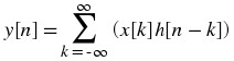 As with continuous-time, convolution is represented by the symbol *, and can be written as y[n] = x[n] * h[n] Convolution is commutative. For more information on the characteristics of convolution, read about the Properties of Convolution.
Convolution Theorem
Let f and g be two functions with convolution f * g .. Let F be the Fourier transform operator. Then
(9.7)F ( f * g ) = F ( f ) · F ( g )
(9.8)F ( f · g ) = F ( f ) * F ( g )
By applying the inverse Fourier transform F – 1 , we can write:
(9.9)f * g = F – 1 ( F ( f ) · F ( g ) )
Conclusion
The Fourier transform of a convolution is the pointwise product of Fourier transforms. In other words, convolution in one domain (e.g., time domain) corresponds to point-wise multiplication in the other domain (e.g., frequency domain).
Chapter 10. Sampling and Reconstruction
10.1. Signal Sampling*
Introduction
Digital computers can process discrete time signals using extremely flexible and powerful algorithms. However, most signals of interest are continuous time signals, which is how data almost always appears in nature. This module introduces the concepts behind converting continuous time signals into discrete time signals through a process called sampling.
Sampling
Sampling a continuous time signal produces a discrete time signal by selecting the values of the continuous time signal at evenly spaced points in time. Thus, sampling a continuous time signal x with sampling period T
s
gives the discrete time signal x
s
defined by 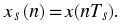 The sampling angular frequency is then given by ω
s
= 2π / T
s
.
The sampling angular frequency is then given by ω
s
= 2π / T
s
.
It should be intuitively clear that multiple continuous time signals sampled at the same rate can produce the same discrete time signal since uncountably many continuous time functions could be constructed that connect the points on the graph of any discrete time function. Thus, sampling at a given rate does not result in an injective relationship. Hence, sampling is, in general, not invertible.
Example 10.1.
For instance, consider the signals x,y defined by
(10.1)

(10.2)
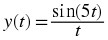
and their sampled versions x S ,y s with sampling period T s = π / 2
(10.3)
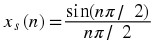
(10.4)
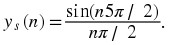
Notice that since
(10.5) sin ( n 5 π / 2 ) = sin ( n 2 π + n π / 2 ) = sin ( n π / 2 )
it follows that
(10.6)
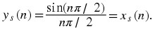
Hence, x and y provide an example of distinct functions with the same sampled versions at a specific sampling rate.
It is also useful to consider the relationship between the frequency domain representations of the continuous time function and its sampled versions. Consider a signal x sampled with sampling period T
s
to produce the discrete time signal  . The spectrum X
s
(ω) for ω ∈ [ – π,π) of x
s
is given by
. The spectrum X
s
(ω) for ω ∈ [ – π,π) of x
s
is given by
(10.7)
Using the continuous time Fourier transform,  can be represented as
(10.8)

Thus, the unit sampling period version of  , which is
  can be represented as
(10.9)
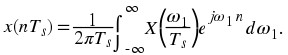
This is algebraically equivalent to the representation
(10.10)
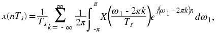
which reduces by periodicity of complex exponentials to
(10.11)
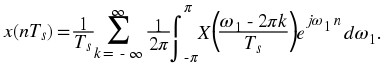
Hence, it follows that
(10.12)
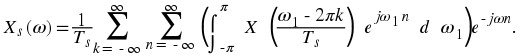
Noting that the above expression contains a Fourier series and inverse Fourier series pair, it follows that
(10.13)

Hence, the spectrum of the sampled signal is, intuitively, the scaled sum of an infinite number of shifted and time scaled copies of original signal spectrum. Aliasing, which will be discussed in depth in later modules, occurs when these shifted spectrum copies overlap and sum together. Note that when the original signal x is bandlimited to  no overlap occurs, so each period of the sampled signal spectrum has the same form as the orignal signal spectrum. This suggest that if we sample a bandlimited signal at a sufficiently high sampling rate, we can recover it from its samples as will be further described in the modules on the Nyquist-Shannon sampling theorem and on perfect reconstruction.
Sampling Summary
Sampling a continuous time signal produces a discrete time signal by selecting the values of the continuous time signal at equally spaced points in time. However, we have shown that this relationship is not injective as multiple continuous time signals can be sampled at the same rate to produce the same discrete time signal. This is related to a phenomenon called aliasing which will be discussed in later modules. Consequently, the sampling process is not, in general, invertible. Nevertheless, as will be shown in the module concerning reconstruction, the continuous time signal can be recovered from its sampled version if some additional assumptions hold.
10.2. Sampling Theorem*
Introduction
With the introduction of the concept of signal sampling, which produces a discrete time signal by selecting the values of the continuous time signal at evenly spaced points in time, it is now possible to discuss one of the most important results in signal processing, the Nyquist-Shannon sampling theorem. Often simply called the sampling theorem, this theorem concerns signals, known as bandlimited signals, with spectra that are zero for all frequencies with absolute value greater than or equal to a certain level. The theorem implies that there is a sufficiently high sampling rate at which a bandlimited signal can be recovered exactly from its samples, which is an important step in the processing of continuous time signals using the tools of discrete time signal processing.
Nyquist-Shannon Sampling Theorem
Statement of the Sampling Theorem
The Nyquist-Shannon sampling theorem concerns signals with continuous time Fourier transforms that are only nonzero on the interval ( – B,B) for some constant B . Such a function is said to be bandlimited to ( – B,B). Essentially, the sampling theorem has already been implicitly introduced in the previous module concerning sampling. Given a continuous time signals x with continuous time Fourier transform X , recall that the spectrum X s of sampled signal x s with sampling period T s is given by
(10.14)

It had previously been noted that if x is bandlimited to  , the period of X
s
centered about the origin has the same form as X scaled in frequency since no aliasing occurs. This is illustrated in Figure 10.1. Hence, if any two
, the period of X
s
centered about the origin has the same form as X scaled in frequency since no aliasing occurs. This is illustrated in Figure 10.1. Hence, if any two  bandlimited continuous time signals sampled to the same signal, they would have the same continuous time Fourier transform and thus be identical. Thus, for each discrete time signal there is a unique
  bandlimited continuous time signal that samples to the discrete time signal with sampling period T
s
. Therefore, this
bandlimited continuous time signal that samples to the discrete time signal with sampling period T
s
. Therefore, this  bandlimited signal can be found from the samples by inverting this bijection.
This is the essence of the sampling theorem. More formally, the sampling theorem states the following. If a signal x is bandlimited to ( – B,B), it is completely determined by its samples with sampling rate ω s = 2B . That is to say, x can be reconstructed exactly from its samples x s with sampling rate ω s = 2B . The angular frequency 2B is often called the angular Nyquist rate. Equivalently, this can be stated in terms of the sampling period T s = 2π / ω s . If a signal x is bandlimited to ( – B,B), it is completely determined by its samples with sampling period T s = π / B . That is to say, x can be reconstructed exactly from its samples x s with sampling period T s .
Figure 10.1.

The spectrum of a bandlimited signals is shown as well as the spectra of its samples at rates above and below the Nyquist frequency. As is shown, no aliasing occurs above the Nyquist frequency, and the period of the samples spectrum centered about the origin has the same form as the spectrum of the original signal scaled in frequency. Below the Nyquist frequency, aliasing can occur and causes the spectrum to take a different than the original spectrum.
Proof of the Sampling Theorem
The above discussion has already shown the sampling theorem in an informal and intuitive way that could easily be refined into a formal proof. However, the original proof of the sampling theorem, which will be given here, provides the interesting observation that the samples of a signal with period T
s
provide Fourier series coefficients for the original signal spectrum on  .
.
Let x be a  bandlimited signal and x
s
be its samples with sampling period T
s
. We can represent x in terms of its spectrum X using the inverse continuous time Fourier transfrom and the fact that x is bandlimited. The result is
bandlimited signal and x
s
be its samples with sampling period T
s
. We can represent x in terms of its spectrum X using the inverse continuous time Fourier transfrom and the fact that x is bandlimited. The result is
(10.15)
This representation of x may then be sampled with sampling period T s to produce
(10.16)
Noticing that this indicates that x
s
(n) is the n th continuous time Fourier series coefficient for X(ω) on the interval  , it is shown that the samples determine the original spectrum X(ω) and, by extension, the original signal itself.
Perfect Reconstruction
Another way to show the sampling theorem is to derive the reconstruction formula that gives the original signal  from its samples x
s
with sampling period T
s
, provided x is bandlimited to
from its samples x
s
with sampling period T
s
, provided x is bandlimited to  . This is done in the module on perfect reconstruction. However, the result, known as the Whittaker-Shannon reconstruction formula, will be stated here. If the requisite conditions hold, then the perfect reconstruction is given by
(10.17)
where the sinc function is defined as
(10.18)

From this, it is clear that the set
(10.19)

forms an orthogonal basis for the set of  bandlimited signals, where the coefficients of a
  signal in this basis are its samples with sampling period T
s
.
signal in this basis are its samples with sampling period T
s
.
Practical Implications
Discrete Time Processing of Continuous Time Signals
The Nyquist-Shannon Sampling Theorem and the Whittaker-Shannon Reconstruction formula enable discrete time processing of continuous time signals. Because any linear time invariant filter performs a multiplication in the frequency domain, the result of applying a linear time invariant filter to a bandlimited signal is an output signal with the same bandlimit. Since sampling a bandlimited continuous time signal above the Nyquist rate produces a discrete time signal with a spectrum of the same form as the original spectrum, a discrete time filter could modify the samples spectrum and perfectly reconstruct the output to produce the same result as a continuous time filter. This allows the use of digital computing power and flexibility to be leveraged in continuous time signal processing as well. This is more thouroughly described in the final module of this chapter.
Psychoacoustics
The properties of human physiology and psychology often inform design choices in technologies meant for interactin with people. For instance, digital devices dealing with sound use sampling rates related to the frequency range of human vocalizations and the frequency range of human auditory sensativity. Because most of the sounds in human speech concentrate most of their signal energy between 5 Hz and 4 kHz, most telephone systems discard frequencies above 4 kHz and sample at a rate of 8 kHz. Discarding the frequencies greater than or equal to 4 kHz through use of an anti-aliasing filter is important to avoid aliasing, which would negatively impact the quality of the output sound as is described in a later module. Similarly, human hearing is sensitive to frequencies between 20 Hz and 20 kHz. Therefore, sampling rates for general audio waveforms placed on CDs were chosen to be greater than 40 kHz, and all frequency content greater than or equal to some level is discarded. The particular value that was chosen, 44.1 kHz, was selected for other reasons, but the sampling theorem and the range of human hearing provided a lower bound for the range of choices.
Sampling Theorem Summary
The Nyquist-Shannon Sampling Theorem states that a signal bandlimited to  can be reconstructed exactly from its samples with sampling period T
s
. The Whittaker-Shannon interpolation formula, which will be further described in the section on perfect reconstruction, provides the reconstruction of the unique
can be reconstructed exactly from its samples with sampling period T
s
. The Whittaker-Shannon interpolation formula, which will be further described in the section on perfect reconstruction, provides the reconstruction of the unique  bandlimited continuous time signal that samples to a given discrete time signal with sampling period T
s
. This enables discrete time processing of continuous time signals, which has many powerful applications.
bandlimited continuous time signal that samples to a given discrete time signal with sampling period T
s
. This enables discrete time processing of continuous time signals, which has many powerful applications.
10.3. Signal Reconstruction*
Introduction
The sampling process produces a discrete time signal from a continuous time signal by examining the value of the continuous time signal at equally spaced points in time. Reconstruction, also known as interpolation, attempts to perform an opposite process that produces a continuous time signal coinciding with the points of the discrete time signal. Because the sampling process for general sets of signals is not invertible, there are numerous possible reconstructions from a given discrete time signal, each of which would sample to that signal at the appropriate sampling rate. This module will introduce some of these reconstruction schemes.
Reconstruction
Reconstruction Process
The process of reconstruction, also commonly known as interpolation, produces a continuous time signal that would sample to a given discrete time signal at a specific sampling rate. Reconstruction can be mathematically understood by first generating a continuous time impulse train
(10.20)
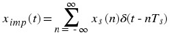
from the sampled signal x
s
with sampling period T
s
and then applying a lowpass filter G that satisfies certain conditions to produce an output signal  . If G has impulse response g , then the result of the reconstruction process, illustrated in Figure 10.2, is given by the following computation, the final equation of which is used to perform reconstruction in practice.
(10.21)
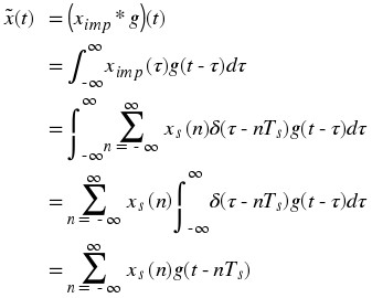
Figure 10.2.
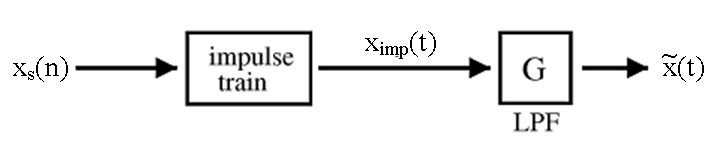
Block diagram of reconstruction process for a given lowpass filter G .
Reconstruction Filters
In order to guarantee that the reconstructed signal  samples to the discrete time signal x
s
from which it was reconstructed using the sampling period T
s
, the lowpass filter G must satisfy certain conditions. These can be expressed well in the time domain in terms of a condition on the impulse response g of the lowpass filter G . The sufficient condition to be a reconstruction filters that we will require is that, for all n ∈ Z,
samples to the discrete time signal x
s
from which it was reconstructed using the sampling period T
s
, the lowpass filter G must satisfy certain conditions. These can be expressed well in the time domain in terms of a condition on the impulse response g of the lowpass filter G . The sufficient condition to be a reconstruction filters that we will require is that, for all n ∈ Z,
(10.22)

This means that g sampled at a rate T
s
produces a discrete time unit impulse signal. Therefore, it follows that sampling  with sampling period T
s
results in
with sampling period T
s
results in
(10.23)
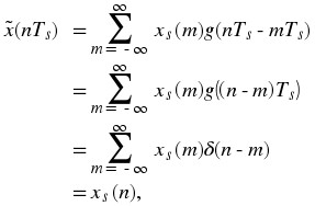
which is the desired result for reconstruction filters.
Cardinal Basis Splines
Since there are many continuous time signals that sample to a given discrete time signal, additional constraints are required in order to identify a particular one of these. For instance, we might require our reconstruction to yield a spline of a certain degree, which is a signal described in piecewise parts by polynomials not exceeding that degree. Additionally, we might want to guarantee that the function and a certain number of its derivatives are continuous.
This may be accomplished by restricting the result to the span of sets of certain splines, called basis splines or B-splines. Specifically, if a n th degree spline with continuous derivatives up to at least order n – 1 is required, then the desired function for a given T
s
belongs to the span of 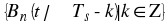 where
where
(10.24)B n = B 0 * B n – 1
for n ≥ 1 and
(10.25)
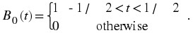
Figure 10.3.
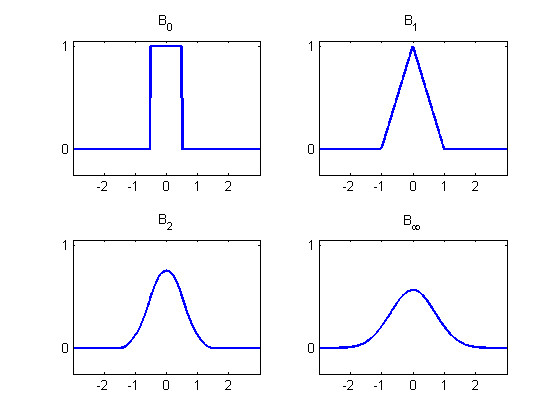
The basis splines B n are shown in the above plots. Note that, except for the order 0 and order 1 functions, these functions do not satisfy the conditions to be reconstruction filters. Also notice that as the order increases, the functions approach the Gaussian function, which is exactly B ∞ .
However, the basis splines B n do not satisfy the conditions to be a reconstruction filter for n ≥ 2 as is shown in Figure 10.3. Still, the B n are useful in defining the cardinal basis splines, which do satisfy the conditions to be reconstruction filters. If we let b n be the samples of B n on the integers, it turns out that b n has an inverse b n – 1 with respect to the operation of convolution for each n . This is to say that b n – 1 * b n = δ . The cardinal basis spline of order n for reconstruction with sampling period T s is defined as
(10.26)
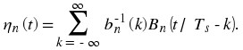
In order to confirm that this satisfies the condition to be a reconstruction filter, note that
(10.27)
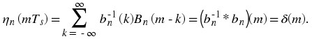
Thus, η n is a valid reconstruction filter. Since η n is an n th degree spline with continuous derivatives up to order n – 1, the result of the reconstruction will be a n th degree spline with continuous derivatives up to order n – 1.
Figure 10.4.
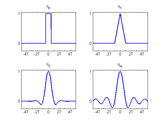
The above plots show cardinal basis spline functions η 0 , η 1 , η 2 , and η ∞ . Note that the functions satisfy the conditions to be reconstruction filters. Also, notice that as the order increases, the cardinal basis splines approximate the sinc function, which is exactly η ∞ . Additionally, these filters are acausal.
The lowpass filter with impulse response equal to the cardinal basis spline η 0 of order 0 is one of the simplest examples of a reconstruction filter. It simply extends the value of the discrete time signal for half the sampling period to each side of every sample, producing a piecewise constant reconstruction. Thus, the result is discontinuous for all nonconstant discrete time signals.
Likewise, the lowpass filter with impulse response equal to the cardinal basis spline η 1 of order 1 is another of the simplest examples of a reconstruction filter. It simply joins the adjacent samples with a straight line, producing a piecewise linear reconstruction. In this way, the reconstruction is continuous for all possible discrete time signals. However, unless the samples are collinear, the result has discontinuous first derivatives.
In general, similar statements can be made for lowpass filters with impulse responses equal to cardinal basis splines of any order. Using the n th order cardinal basis spline η n , the result is a piecewise degree n polynomial. Furthermore, it has continuous derivatives up to at least order n – 1. However, unless all samples are points on a polynomial of degree at most n , the derivative of order n will be discontinuous.
Reconstructions of the discrete time signal given in Figure 10.5 using several of these filters are shown in Figure 10.6. As the order of the cardinal basis spline increases, notice that the reconstruction approaches that of the infinite order cardinal spline η ∞ , the sinc function. As will be shown in the subsequent section on perfect reconstruction, the filters with impulse response equal to the sinc function play an especially important role in signal processing.
Figure 10.5.
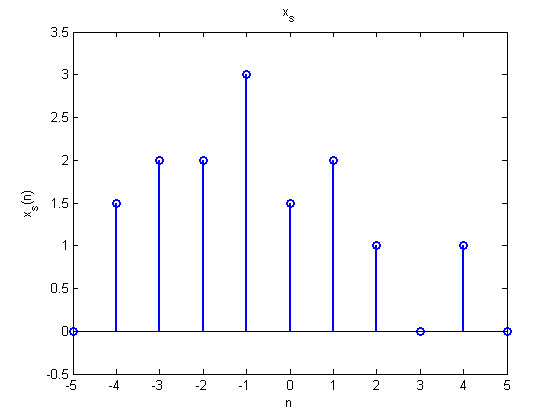
The above plot shows an example discrete time function. This discrete time function will be reconstructed using sampling period T s using several cardinal basis splines in Figure 10.6.
Figure 10.6.
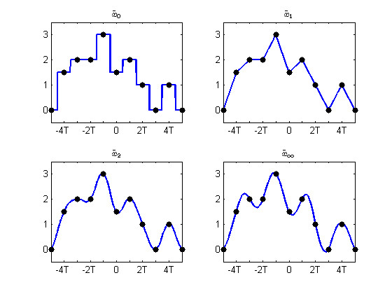
The above plots show interpolations of the discrete time signal given in Figure 10.5 using lowpass filters with impulse responses given by the cardinal basis splines shown in Figure 10.4. Notice that the interpolations become increasingly smooth and approach the sinc interpolation as the order increases.
Reconstruction Summary
Reconstruction of a continuous time signal from a discrete time signal can be accomplished through several schemes. However, it is important to note that reconstruction is not the inverse of sampling and only produces one possible continuous time signal that samples to a given discrete time signal. As is covered in the subsequent module, perfect reconstruction of a bandlimited continuous time signal from its sampled version is possible using the Whittaker-Shannon reconstruction formula, which makes use of the ideal lowpass filter and its sinc function impulse response, if the sampling rate is sufficiently high.
10.4. Perfect Reconstruction*
Introduction
If certain additional assumptions about the original signal and sampling rate hold, then the original signal can be recovered exactly from its samples using a particularly important type of filter. More specifically, it will be shown that if a bandlimited signal is sampled at a rate greater than twice its bandlimit, the Whittaker-Shannon reconstruction formula perfectly reconstructs the original signal. This formula makes use of the ideal lowpass filter, which is related to the sinc function. This is extremely useful, as sampled versions of continuous time signals can be filtered using discrete time signal processing, often in a computer. The results may then be reconstructed to produce the same continuous time output as some desired continuous time system.
Perfect Reconstruction
In order to understand the conditions for perfect reconstruction and the filter it employs, consider the following. As a beginning, a sufficient condition under which perfect reconstruction is possible will be discussed. Subsequently, the filter and process used for perfect reconstruction will be detailed.
Recall that the sampled version x s of a continuous time signal x with sampling period T s has a spectrum given by
(10.28)
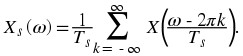
As before, note that if x is bandlimited to  , meaning that X is only nonzero on
  , then each period of X
s
has the same form as X . Thus, we can identify the original spectrum X from the spectrum of the samples X
s
and, by extension, the original signal x from its samples x
s
at rate T
s
if x is bandlimited to
, then each period of X
s
has the same form as X . Thus, we can identify the original spectrum X from the spectrum of the samples X
s
and, by extension, the original signal x from its samples x
s
at rate T
s
if x is bandlimited to 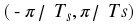 .
.
If a signal x is bandlimited to ( – B,B), then it is also bandlimited to  provided that T
s
< π / B . Thus, if we ensure that x is sampled to x
s
with sufficiently high sampling angular frequency ω
s
= 2π / T
s
> 2B and have a way of identifying the unique
provided that T
s
< π / B . Thus, if we ensure that x is sampled to x
s
with sufficiently high sampling angular frequency ω
s
= 2π / T
s
> 2B and have a way of identifying the unique  bandlimited signal corresponding to a discrete time signal at sampling period T
s
, then x
s
can be used to reconstruct
bandlimited signal corresponding to a discrete time signal at sampling period T
s
, then x
s
can be used to reconstruct  exactly. The frequency 2B is known as the angular Nyquist rate. Therefore, the condition that the sampling rate ω
s
= 2π / T
s
> 2B be greater than the Nyquist rate is a sufficient condition for perfect reconstruction to be possible.
exactly. The frequency 2B is known as the angular Nyquist rate. Therefore, the condition that the sampling rate ω
s
= 2π / T
s
> 2B be greater than the Nyquist rate is a sufficient condition for perfect reconstruction to be possible.
The correct filter must also be known in order to perform perfect reconstruction. The ideal lowpass filter defined by G(ω) = T
s
(u (ω + π / T
s
) – u (ω – π / T
s
)), which is shown in Figure 10.7, removes all signal content not in the frequency range  . Therefore, application of this filter to the impulse train
  results in an output bandlimited to
  .
.
We now only need to confirm that the impulse response g of the filter G satisfies our sufficient condition to be a reconstruction filter. The inverse Fourier transform of G(ω) is
(10.29)

which is shown in Figure 10.7. Hence,
(10.30)
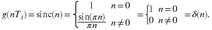
Therefore, the ideal lowpass filter G is a valid reconstruction filter. Since it is a valid reconstruction filter and always produces an output that is bandlimited to  , this filter always produces the unique
  bandlimited signal that samples to a given discrete time sequence at sampling period T
s
when the impulse train
bandlimited signal that samples to a given discrete time sequence at sampling period T
s
when the impulse train 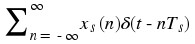 is input.
Therefore, we can always reconstruct any  bandlimited signal from its samples at sampling period T
s
by the formula
bandlimited signal from its samples at sampling period T
s
by the formula
(10.31)
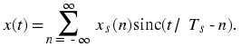
This perfect reconstruction formula is known as the Whittaker-Shannon interpolation formula and is sometimes also called the cardinal series. In fact, the sinc function is the infinite order cardinal basis spline η
∞ . Consequently, the set 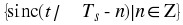 forms a basis for the vector space of
  bandlimited signals where the signal samples provide the corresponding coefficients. It is a simple exercise to show that this basis is, in fact, an orthogonal basis.
Figure 10.7.
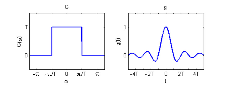
The above plots show the ideal lowpass filter and its inverse Fourier transform, the sinc function.
Figure 10.8.
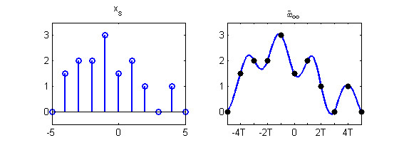
The plots show an example discrete time signal and its Whittaker-Shannon sinc reconstruction.
Perfect Reconstruction Summary
This module has shown that bandlimited continuous time signals can be reconstructed exactly from their samples provided that the sampling rate exceeds the Nyquist rate, which is twice the bandlimit. The Whittaker-Shannon reconstruction formula computes this perfect reconstruction using an ideal lowpass filter, with the resulting signal being a sum of shifted sinc functions that are scaled by the sample values. Sampling below the Nyquist rate can lead to aliasing which makes the original signal irrecoverable as is described in the subsequent module. The ability to perfectly reconstruct bandlimited signals has important practical implications for the processing of continuous time signals using the tools of discrete time signal processing.
10.5. Aliasing Phenomena*
Introduction
Through discussion of the Nyquist-Shannon sampling theorem and Whittaker-Shannon reconstruction formula, it has already been shown that a ( – B,B) continuous time signal can be reconstructed from its samples at rate ω s = 2π / T s via the sinc interpolation filter if ω s > 2B . Now, this module will investigate a problematic phenomenon, called aliasing, that can occur if this sufficient condition for perfect reconstruction does not hold. When aliasing occurs the spectrum of the samples has different form than the original signal spectrum, so the samples cannot be used to reconstruct the original signal through Whittaker-Shannon interpolation.
Aliasing
Aliasing occurs when each period of the spectrum of the samples does not have the same form as the spectrum of the original signal. Given a continuous time signals x with continuous time Fourier transform X , recall that the spectrum X s of sampled signal x s with sampling period T s is given by
(10.32)

As has already been mentioned several times, if x is bandlimited to  then each period of X
s
has the same form as X . However, if x is not bandlimited to
then each period of X
s
has the same form as X . However, if x is not bandlimited to  , then the
  can overlap and sum together. This is illustrated in Figure 10.9 in which sampling above the Nyquist frequency produces a samples spectrum of the same shape as the original signal, but sampling below the Nyquist frequency produces a samples spectrum with very different shape. Whittaker-Shannon interpolation of each of these sequences produces different results. The low frequencies not affected by the overlap are the same, but there is noise content in the higher frequencies caused by aliasing. Higher frequency energy masquerades as low energy content, a highly undesirable effect.
Figure 10.9.
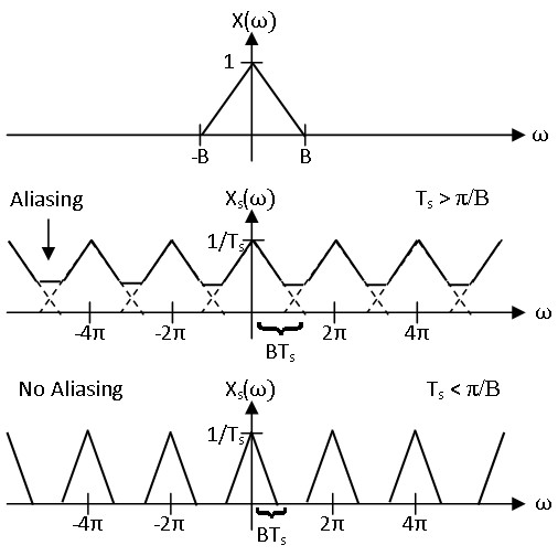
The spectrum of a bandlimited signals is shown as well as the spectra of its samples at rates above and below the Nyquist frequency. As is shown, no aliasing occurs above the Nyquist frequency, and the period of the samples spectrum centered about the origin has the same form as the spectrum of the original signal scaled in frequency. Below the Nyquist frequency, aliasing can occur and causes the spectrum to take a different than the original spectrum.
Unlike when sampling above the Nyquist frequency, sampling below the Nyquist frequency does not yield an injective (one-to-one) function from the ( – B,B) bandlimited continuous time signals to the discrete time signals. Any signal x with spectrum X which overlaps and sums to X s samples to x s . It should be intuitively clear that there are very many ( – B,B) bandlimited signals that sample to a given discrete time signal below the Nyquist frequency, as is demonstrated in Figure 10.10. It is quite easy to construct uncountably infinite families of such signals.
Aliasing obtains it name from the fact that multiple, in fact infinitely many, ( – B,B) bandlimited signals sample to the same discrete sequence if ω
s
< 2B . Thus, information about the original signal is lost in this noninvertible process, and these different signals effectively assume the same identity, an “alias”. Hence, under these conditions the Whittaker-Shannon interpolation formula will not produce a perfect reconstruction of the original signal but will instead give the unique  bandlimited signal that samples to the discrete sequence.
Figure 10.10.
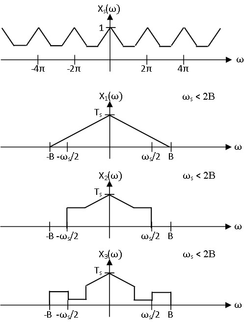
The spectrum of a discrete time signal x s , taken from Figure 10.9, is shown along with the spectra of three ( – B,B) signals that sample to it at rate ω s < 2B . From the sampled signal alone, it is impossible to tell which, if any, of these was sampled at rate ω s to produce x s . In fact, there are infinitely many ( – B,B) bandlimited signals that sample to x s at a sampling rate below the Nyquist rate.
Aliasing Demonstration
Figure 10.11.
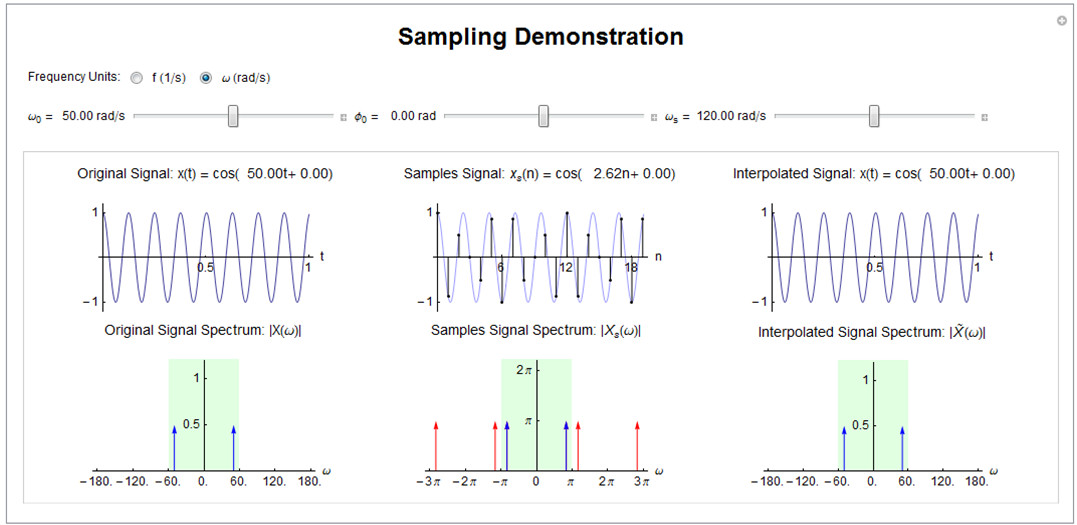
Interact (when online) with a Mathematica CDF demonstrating sampling and aliasing for a sinusoid. To Download, right-click and save target as .cdf.
Aliasing Summary
Aliasing, essentially the signal processing version of identity theft, occurs when each period of the spectrum of the samples does not have the same form as the spectrum of the original signal. As has been shown, there can be infinitely many ( – B,B) bandlimited signals that sample to a given discrete time signal x s at a rate ω s = 2π / T s < 2B below the Nyquist frequency. However, there is a unique ( – B,B) bandlimited signal that samples to x s , which is given by the Whittaker-Shannon interpolation of x s , at rate ω s ≥ 2B as no aliasing occurs above the Nyquist frequency. Unfortunately, sufficiently high sampling rates cannot always be produced. Aliasing is detrimental to many signal processing applications, so in order to process continuous time signals using discrete time tools, it is often necessary to find ways to avoid it other than increasing the sampling rate. Thus, anti-aliasing filters, are of practical importance.
10.6. Anti-Aliasing Filters*
Introduction
It has been shown that a ( – B,B) bandlimited signal can be perfectly reconstructed from its samples at a rate ω
s
= 2π / T
s
≥ B . However, it is not always practically possible to produce sufficiently high sampling rates or to ensure that the input is bandlimited in real situations. Aliasing, which manifests itself as a difference in shape between the periods of the samples signal spectrum and the original spectrum, would occur without any further measures to correct this. Thus, it often becomes necessary to filter out signal energy at frequencies above ω
s
/ 2 in order to avoid the detrimental effects of aliasing. This is the role of the anti-aliasing filter, a lowpass filter applied before sampling to ensure that the signal is  bandlimited or at least nearly so.
Anti-Aliasing Filters
Aliasing can occur when a signal with energy at frequencies other that ( – B,B) is sampled at rate ω s < 2B . Thus, when sampling below the Nyquist frequency, it is desirable to remove as much signal energy outside the frequency range ( – B,B) as possible while keeping as much signal energy in the frequency range ( – B,B) as possible. This suggests that the ideal lowpass filter with cutoff frequency ω s / 2 would be the optimal anti-aliasing filter to apply before sampling. While this is true, the ideal lowpass filter can only be approximated in real situations.
In order to demonstrate the importance of anti-aliasing filters, consider the calculation of the error energy between the original signal and its Whittaker-Shannon reconstruction from its samples taken with and without the use of an anti-aliasing filter. Let x be the original signal and y = G x be the anti-alias filtered signal where G is the ideal lowpass filter with cutoff frequency ω s / 2. It is easy to show that the reconstructed spectrum using no anti-aliasing filter is given by
(10.33)
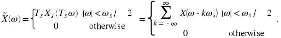
Thus, the reconstruction error spectrum for this case is
(10.34)
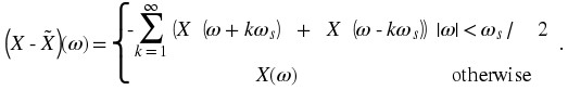
Similarly, the reconstructed spectrum using the ideal lowpass anti-aliasing filter is given by
(10.35)
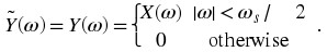
Thus, the reconstruction error spectrum for this case is
(10.36)
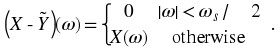
Hence, by Parseval's theorem, it follows that 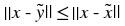 . Also note that the spectrum of
  is identical to that of the original signal X at frequencies
 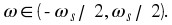 This is graphically shown in Figure 10.12.
Figure 10.12.

The figure above illustrates the use of an anti-aliasing filter to improve the process of sampling and reconstruction when using a sampling frequency below the Nyquist frequency. Notice that when using an ideal lowpass anti-aliasing filter, the reconstructed signal spectrum has the same shape as the original signal spectrum for all frequencies below half the sampling rate. This results in a lower error energy when using the anti-aliasing filter, as can be seen by comparing the error spectra shown.
Anti-Aliasing Filters Summary
As can be seen, anti-aliasing filters ensure that the signal is  bandlimited, or at least nearly so. The optimal anti-aliasing filter would be the ideal lowpass filter with cutoff frequency at ω
s
/ 2, which would ensure that the original signal spectrum and the reconstructed signal spectrum are equal on the interval
bandlimited, or at least nearly so. The optimal anti-aliasing filter would be the ideal lowpass filter with cutoff frequency at ω
s
/ 2, which would ensure that the original signal spectrum and the reconstructed signal spectrum are equal on the interval  . However, the ideal lowpass filter is not possible to implement in practice, and approximations must be accepted instead. Anti-aliasing filters are an important component of systems that implement discrete time processing of continuous time signals, as will be shown in the subsequent module.
10.7. Discrete Time Processing of Continuous Time Signals*
Introduction
Digital computers can process discrete time signals using extremely flexible and powerful algorithms. However, most signals of interest are continuous time signals, which is how data almost always appears in nature. Now that the theory supporting methods for generating a discrete time signal from a continuous time signal through sampling and then perfectly reconstructing the original signal from its samples without error has been discussed, it will be shown how this can be applied to implement continuous time, linear time invariant systems using discrete time, linear time invariant systems. This is of key importance to many modern technologies as it allows the power of digital computing to be leveraged for processing of analog signals.
Discrete Time Processing of Continuous Time Signals
Process Structure
With the aim of processing continuous time signals using a discrete time system, we will now examine one of the most common structures of digital signal processing technologies. As an overview of the approach taken, the original continuous time signal x is sampled to a discrete time signal x s in such a way that the periods of the samples spectrum X s is as close as possible in shape to the spectrum of X . Then a discrete time, linear time invariant filter H 2 is applied, which modifies the shape of the samples spectrum X s but cannot increase the bandlimit of X s , to produce another signal y s . This is reconstructed with a suitable reconstruction filter to produce a continuous time output signal y , thus effectively implementing some continuous time system H 1 . This process is illustrated in Figure 10.13, and the spectra are shown for a specific case in Figure 10.14.
Figure 10.13.
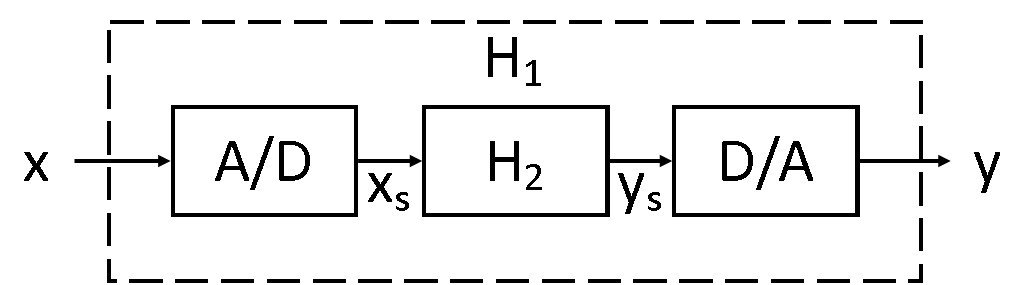
A block diagram for processing of continuous time signals using discrete time systems is shown.
Further discussion about each of these steps is necessary, and we will begin by discussing the analog to digital converter, often denoted by ADC or A/D. It is clear that in order to process a continuous time signal using discrete time techniques, we must sample the signal as an initial step. This is essentially the purpose of the ADC, although there are practical issues that which will be discussed later. An ADC takes a continuous time analog signal as input and produces a discrete time digital signal as output, with the ideal infinite precision case corresponding to sampling. As stated by the Nyquist-Shannon Sampling theorem, in order to retain all information about the original signal, we usually wish sample above the Nyquist frequency ω s ≥ 2B where the original signal is bandlimited to ( – B,B). When it is not possible to guarantee this condition, an anti-aliasing filter should be used.
The discrete time filter is where the intentional modifications to the signal information occur. This is commonly done in digital computer software after the signal has been sampled by a hardware ADC and before it is used by a hardware DAC to construct the output. This allows the above setup to be quite flexible in the filter that it implements. If sampling above the Nyquist frequency the. Any modifications that the discrete filter makes to this shape can be passed on to a continuous time signal assuming perfect reconstruction. Consequently, the process described will implement a continuous time, linear time invariant filter. This will be explained in more mathematical detail in the subsequent section. As usual, there are, of course, practical limitations that will be discussed later.
Finally, we will discuss the digital to analog converter, often denoted by DAC or D/A. Since continuous time filters have continuous time inputs and continuous time outputs, we must construct a continuous time signal from our filtered discrete time signal. Assuming that we have sampled a bandlimited at a sufficiently high rate, in the ideal case this would be done using perfect reconstruction through the Whittaker-Shannon interpolation formula. However, there are, once again, practical issues that prevent this from happening that will be discussed later.
Figure 10.14.
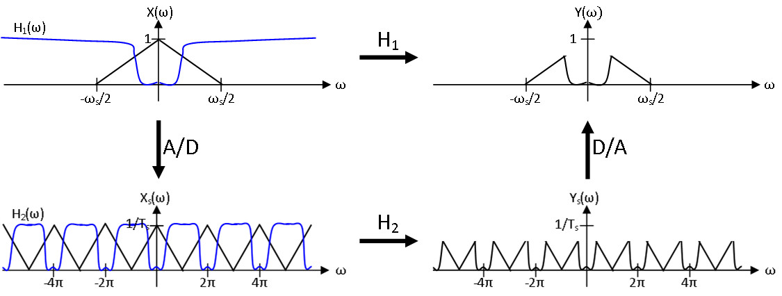
Spectra are shown in black for each step in implementing a continuous time filter using a discrete time filter for a specific signal. The filter frequency responses are shown in blue, and both are meant to have maximum value 1 in spite of the vertical scale that is meant only for the signal spectra. Ideal ADCs and DACs are assumed.
Discrete Time Filter
With some initial discussion of the process illustrated in Figure 10.13 complete, the relationship between the continuous time, linear time invariant filter H 1 and the discrete time, linear time invariant filter H 2 can be explored. We will assume the use of ideal, infinite precision ADCs and DACs that perform sampling and perfect reconstruction, respectively, using a sampling rate ω s = 2π / T s ≥ 2B where the input signal x is bandlimited to ( – B,B). Note that these arguments fail if this condition is not met and aliasing occurs. In that case, preapplication of an anti-aliasing filter is necessary for these arguments to hold.
Recall that we have already calculated the spectrum X s of the samples x s given an input x with spectrum X as
(10.37)

Likewise, the spectrum Y s of the samples y s given an output y with spectrum Y is
(10.38)

From the knowledge that  , it follows that
(10.39)
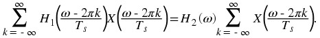
Because X is bandlimited to  , we may conclude that
(10.40)

More simply stated, H
2 is 2π periodic and  for ω ∈ [ – π,π).
Given a specific continuous time, linear time invariant filter H
1 , the above equation solves the system design problem provided we know how to implement H
2 . The filter H
2 must be chosen such that it has a frequency response where each period has the same shape as the frequency response of H
1 on  . This is illustrated in the frequency responses shown in Figure 10.14.
We might also want to consider the system analysis problem in which a specific discrete time, linear time invariant filter H
2 is given, and we wish to describe the filter H
1 . There are many such filters, but we can describe their frequency responses on  using the above equation. Isolating one period of H
2(ω) yields the conclusion that
using the above equation. Isolating one period of H
2(ω) yields the conclusion that  for
for  . Because x was assumed to be bandlimited to ( – π / T,π / T), the value of the frequency response elsewhere is irrelevant.
Practical Considerations
As mentioned before, there are several practical considerations that need to be addressed at each stage of the process shown in Figure 10.13. Some of these will be briefly addressed here, and a more complete model of how discrete time processing of continuous time signals appears in Figure 10.15.
Figure 10.15.

A more complete model of how discrete time processing of continuous time signals is implemented in practice. Notice the addition of anti-aliasing and anti-imaging filters to promote input and output bandlimitedness. The ADC is shown to perform sampling with quantization. The digital filter is further specified to be causal. The DAC is shown to perform imperfect reconstruction, a zero order hold in this case.
Anti-Aliasing Filter
In reality, we cannot typically guarantee that the input signal will have a specific bandlimit, and sufficiently high sampling rates cannot necessarily be produced. Since it is imperative that the higher frequency components not be allowed to masquerade as lower frequency components through aliasing, anti-aliasing filters with cutoff frequency less than or equal to ω s / 2 must be used before the signal is fed into the ADC. The block diagram in Figure 10.15 reflects this addition.
As described in the previous section, an ideal lowpass filter removing all energy at frequencies above ω s / 2 would be optimal. Of course, this is not achievable, so approximations of the ideal lowpass filter with low gain above ω s / 2 must be accepted. This means that some aliasing is inevitable, but it can be reduced to a mostly insignificant level.
Signal Quantization
In our preceding discussion of discrete time processing of continuous time signals, we had assumed an ideal case in which the ADC performs sampling exactly. However, while an ADC does convert a continuous time signal to a discrete time signal, it also must convert analog values to digital values for use in a digital logic device, a phenomenon called quantization. The ADC subsystem of the block diagram in Figure 10.15 reflects this addition.
The data obtained by the ADC must be stored in finitely many bits inside a digital logic device. Thus, there are only finitely many values that a digital sample can take, specifically 2N where N is the number of bits, while there are uncountably many values an analog sample can take. Hence something must be lost in the quantization process. The result is that quantization limits both the range and precision of the output of the ADC. Both are finite, and improving one at constant number of bits requires sacrificing quality in the other.
Filter Implementability
In real world circumstances, if the input signal is a function of time, the future values of the signal cannot be used to calculate the output. Thus, the digital filter H 2 and the overall system H 1 must be causal. The filter annotation in Figure 10.15 reflects this addition. If the desired system is not causal but has impulse response equal to zero before some time t 0 , a delay can be introduced to make it causal. However, if this delay is excessive or the impulse response has infinite length, a windowing scheme becomes necessary in order to practically solve the problem. Multiplying by a window to decrease the length of the impulse response can reduce the necessary delay and decrease computational requirements.
Take, for instance the case of the ideal lowpass filter. It is acausal and infinite in length in both directions. Thus, we must satisfy ourselves with an approximation. One might suggest that these approximations could be achieved by truncating the sinc impulse response of the lowpass filter at one of its zeros, effectively windowing it with a rectangular pulse. However, doing so would produce poor results in the frequency domain as the resulting convolution would significantly spread the signal energy. Other windowing functions, of which there are many, spread the signal less in the frequency domain and are thus much more useful for producing these approximations.
Anti-Imaging Filter
In our preceding discussion of discrete time processing of continuous time signals, we had assumed an ideal case in which the DAC performs perfect reconstruction. However, when considering practical matters, it is important to remember that the sinc function, which is used for Whittaker-Shannon interpolation, is infinite in length and acausal. Hence, it would be impossible for an DAC to implement perfect reconstruction.
Instead, the DAC implements a causal zero order hold or other simple reconstruction scheme with respect to the sampling rate ω
s
used by the ADC. However, doing so will result in a function that is not bandlimited to  . Therefore, an additional lowpass filter, called an anti-imaging filter, must be applied to the output. The process illustrated in Figure 10.15 reflects these additions. The anti-imaging filter attempts to bandlimit the signal to
  , so an ideal lowpass filter would be optimal. However, as has already been stated, this is not possible. Therefore, approximations of the ideal lowpass filter with low gain above ω
s
/ 2 must be accepted. The anti-imaging filter typically has the same characteristics as the anti-aliasing filter.
, so an ideal lowpass filter would be optimal. However, as has already been stated, this is not possible. Therefore, approximations of the ideal lowpass filter with low gain above ω
s
/ 2 must be accepted. The anti-imaging filter typically has the same characteristics as the anti-aliasing filter.
Discrete Time Processing of Continuous Time Signals Summary
As has been show, the sampling and reconstruction can be used to implement continuous time systems using discrete time systems, which is very powerful due to the versatility, flexibility, and speed of digital computers. However, there are a large number of practical considerations that must be taken into account when attempting to accomplish this, including quantization noise and anti-aliasing in the analog to digital converter, filter implementability in the discrete time filter, and reconstruction windowing and associated issues in the digital to analog converter. Many modern technologies address these issues and make use of this process.
Chapter 11. Laplace Transform and Continuous Time System Design
11.1. Laplace Transform*
Introduction
The Laplace transform is a generalization of the Continuous-Time Fourier Transform. It is used because the CTFT does not converge/exist for many important signals, and yet it does for the Laplace-transform (e.g., signals with infinite l 2 norm). It is also used because it is notationally cleaner than the CTFT. However, instead of using complex exponentials of the form ⅇ ⅈωt , with purely imaginary parameters, the Laplace transform uses the more general, ⅇ st , where s = σ + ⅈω is complex, to analyze signals in terms of exponentially weighted sinusoids.
The Laplace Transform
Bilateral Laplace Transform Pair
Although Laplace transforms are rarely solved in practice using integration (tables and computers (e.g. Matlab) are much more common), we will provide the bilateral Laplace transform pair here for purposes of discussion and derivation. These define the forward and inverse Laplace transformations. Notice the similarities between the forward and inverse transforms. This will give rise to many of the same symmetries found in Fourier analysis.
(11.1)
Laplace Transform

(11.2)
Inverse Laplace Transform
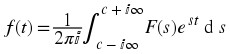
Note
We have defined the bilateral Laplace transform. There is also a unilateral Laplace transform ,
(11.3)
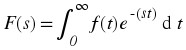
which is useful for solving the difference equations with nonzero initial conditions. This is similar to the unilateral Z Transform in Discrete time.
Relation between Laplace and CTFT
Taking a look at the equations describing the Z-Transform and the Discrete-Time Fourier Transform:
(11.4)
Continuous-Time Fourier Transform
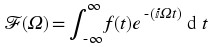
(11.5)
Laplace Transform
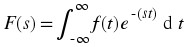
We can see many similarities; first, that : ℱ(Ω) = F(s) for all Ω = s
Note
the CTFT is a complex-valued function of a real-valued variable ω (and 2 π periodic). The Z-transform is a complex-valued function of a complex valued variable z.
Figure 11.1. Plots

Visualizing the Laplace Transform
With the Fourier transform, we had a complex-valued function of a purely imaginary variable, F(ⅈω) . This was something we could envision with two 2-dimensional plots (real and imaginary parts or magnitude and phase). However, with Laplace, we have a complex-valued function of a complex variable. In order to examine the magnitude and phase or real and imaginary parts of this function, we must examine 3-dimensional surface plots of each component.
Figure 11.2. real and imaginary sample plots
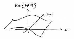
(a) The Real part of H(s)
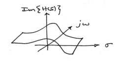
(b) The Imaginary part of H(s)
Real and imaginary parts of H(s) are now each 3-dimensional surfaces.
Figure 11.3. magnitude and phase sample plots
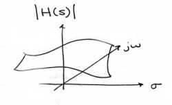
(a) The Magnitude of H(s)
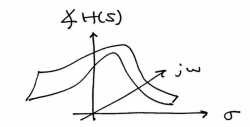
(b) The Phase of H(s)
Magnitude and phase of H(s) are also each 3-dimensional surfaces. This representation is more common than real and imaginary parts.
While these are legitimate ways of looking at a signal in the Laplace domain, it is quite difficult to draw and/or analyze. For this reason, a simpler method has been developed. Although it will not be discussed in detail here, the method of Poles and Zeros is much easier to understand and is the way both the Laplace transform and its discrete-time counterpart the Z-transform are represented graphically.
Using a Computer to find the Laplace Transform
Using a computer to find Laplace transforms is relatively painless. Matlab has two functions, laplace and ilaplace, that are both part of the symbolic toolbox, and will find the Laplace and inverse Laplace transforms respectively. This method is generally preferred for more complicated functions. Simpler and more contrived functions are usually found easily enough by using tables.
Laplace Transform Definition Demonstration
Figure 11.4.
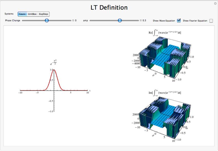
Interact (when online) with a Mathematica CDF demonstrating the Laplace Transform. To Download, right-click and save target as .cdf.
Interactive Demonstrations
Figure 11.5. Khan Lecture on Laplace
(This media type is not supported in this reader. Click to open media in browser.)
See the attached video on the basics of the Unilateral Laplace Transform from Khan Academy
Conclusion
The laplace transform proves a useful, more general form of the Continuous Time Fourier Transform. It applies equally well to describing systems as well as signals using the eigenfunction method, and to describing a larger class of signals better described using the pole-zero method.
11.2. Common Laplace Transforms*
| Signal | Laplace Transform | Region of Convergence |
|---|---|---|
| δ(t) | 1 | All s |
| δ(t − T) | ⅇ – (sT) | All s |
| u(t) | 
| Re( s) > 0 |
| – ( u( – t)) | 
| Re( s) < 0 |
| t u(t) | 
| Re( s) > 0 |
| t n u(t) | 
| Re( s) > 0 |
| – ( t n u( – t)) | 
| Re( s) < 0 |
| ⅇ – (λt) u(t) | 
| Re( s) > – λ |
| ( – ( ⅇ – (λt)))u( – t) | 
| Re( s) < – λ |
| t ⅇ – (λt) u(t) | 
| Re( s) > – λ |
| t n ⅇ – (λt) u(t) | 
| Re( s) > – λ |
| – ( t n ⅇ – (λt) u( – t)) | 
| Re( s) < – λ |
| cos( bt)u(t) | 
| Re( s) > 0 |
| sin( bt)u(t) | 
| Re( s) > 0 |
| ⅇ – (at)cos(bt)u(t) | 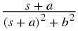
| Re( s) > – a |
| ⅇ – (at)sin(bt)u(t) | 
| Re( s) > – a |

| s n | All s |
11.3. Properties of the Laplace Transform*
| Property | Signal | Laplace Transform | Region of Convergence |
|---|---|---|---|
| Linearity | α x 1(t) + β x 2(t) | α X 1(s) + β X 2(s) | At least ROC 1 ⋂ ROC2 |
| Time Shifting | x(t − τ) | ⅇ – (sτ) X(s) | ROC |
| Frequency Shifting (modulation) | ⅇ ηt x(t) | X(s − η) | Shifted ROC ( s − η must be in the region of convergence) |
| Time Scaling | x(αt) | (1 − | α|)X(s − α) | Scaled ROC ( s − α must be in the region of convergence) |
| Conjugation | 
| 
| ROC |
| Convolution | x 1(t) * x 2(t) | X 1(t)X 2(t) | At least ROC 1 ⋂ ROC2 |
| Time Differentiation | 
| s X(s) | At least ROC |
| Frequency Differentiation | ( – t)x(t) | 
| ROC |
| Integration in Time | 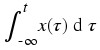
| (1 − s)X(s) | At least ROC ⋂ Re( s) > 0 |
11.4. Inverse Laplace Transform*
Introduction
When using the Laplace-transform
 it is often useful to be able to find h(t) given H(s) . There are at least 4 different methods to do this:
Inspection Method
This "method" is to basically become familiar with the Laplace-transform pair tables and then "reverse engineer".
Example 11.1.
When givenwith an ROC of |s| > α we could determine "by inspection" that h(t) = α t u(t)
Partial-Fraction Expansion Method
When dealing with linear time-invariant systems the z-transform is often of the form 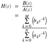 This can also expressed as
 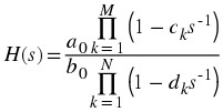 where c
k
represents the nonzero zeros of H(s) and d
k
represents the nonzero poles.
where c
k
represents the nonzero zeros of H(s) and d
k
represents the nonzero poles.
If M < N then H(s) can be represented as 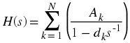 This form allows for easy inversions of each term of the sum using the inspection method and the transform table. If the numerator is a polynomial, however, then it becomes necessary to use partial-fraction expansion to put H(s) in the above form. If M ≥ N then H(s) can be expressed as
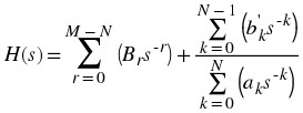
Example 11.2.
Find the inverse z-transform ofwhere the ROC is |s| > 2 . In this case M = N = 2 , so we have to use long division to get
Next factor the denominator.
Now do partial-fraction expansion.
Now each term can be inverted using the inspection method and the Laplace-transform table. Thus, since the ROC is |s| > 2 ,
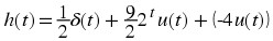
Demonstration of Partial Fraction Expansion
Figure 11.6.
(This media type is not supported in this reader. Click to open media in browser.)
Interactive experiment illustrating how the Partial Fraction Expansion method is used to solve a variety of numerator and denominator problems. (To view and interact with the simulation, download the free Mathematica player at http://www.wolfram.com/products/player/download.cgi)
Figure 11.7. Khan Lecture on Partial Fraction Expansion
(This media type is not supported in this reader. Click to open media in browser.)
video from Khan Academy
Power Series Expansion Method
When the z-transform is defined as a power series in the form 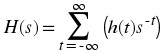 then each term of the sequence h(t) can be determined by looking at the coefficients of the respective power of s
– t
.
then each term of the sequence h(t) can be determined by looking at the coefficients of the respective power of s
– t
.
Example 11.3.
Now look at the Laplace-transform of a finite-length sequence.In this case, since there were no poles, we multiplied the factors of H(s) . Now, by inspection, it is clear that
.
One of the advantages of the power series expansion method is that many functions encountered in engineering problems have their power series' tabulated. Thus functions such as log, sin, exponent, sinh, etc, can be easily inverted.
Example 11.4.
Suppose H(s) = logt (1 + α s -1) Noting thatThen
Therefore

Contour Integration Method
Without going in to much detail 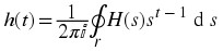 where r is a counter-clockwise contour in the ROC of H(s) encircling the origin of the s-plane. To further expand on this method of finding the inverse requires the knowledge of complex variable theory and thus will not be addressed in this module.
Demonstration of Contour Integration
Figure 11.8.
(This media type is not supported in this reader. Click to open media in browser.)
Interactive experiment illustrating how the contour integral is applied on a simple example. For a more in-depth discussion of this method, some background in complex analysis is required. (To view and interact with the simulation, download the free Mathematica player at http://www.wolfram.com/products/player/download.cgi)
Conclusion
The Inverse Laplace-transform is very useful to know for the purposes of designing a filter, and there are many ways in which to calculate it, drawing from many disparate areas of mathematics. All nevertheless assist the user in reaching the desired time-domain signal that can then be synthesized in hardware(or software) for implementation in a real-world filter.
11.5. Poles and Zeros in the S-Plane*
Introduction to Poles and Zeros of the Laplace-Transform
It is quite difficult to qualitatively analyze the Laplace transform and Z-transform, since mappings of their magnitude and phase or real part and imaginary part result in multiple mappings of 2-dimensional surfaces in 3-dimensional space. For this reason, it is very common to examine a plot of a transfer function's poles and zeros to try to gain a qualitative idea of what a system does.
Once the Laplace-transform of a system has been determined, one can use the information contained in function's polynomials to graphically represent the function and easily observe many defining characteristics. The Laplace-transform will have the below structure, based on Rational Functions: 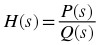
The two polynomials, P(s) and Q(s), allow us to find the poles and zeros of the Laplace-Transform.
Definition: zeros
1. The value(s) for s where.
2. The complex frequencies that make the overall gain of the filter transfer function zero.
Definition: poles
1. The value(s) for s where.
2. The complex frequencies that make the overall gain of the filter transfer function infinite.
Example 11.5.
Below is a simple transfer function with the poles and zeros shown below it.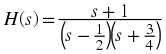
The zeros are: { – 1}
The poles are:
The S-Plane
Once the poles and zeros have been found for a given Laplace Transform, they can be plotted onto the S-Plane. The S-plane is a complex plane with an imaginary and real axis referring to the complex-valued variable z . The position on the complex plane is given by r ⅇ ⅈθ and the angle from the positive, real axis around the plane is denoted by θ . When mapping poles and zeros onto the plane, poles are denoted by an "x" and zeros by an "o". The below figure shows the S-Plane, and examples of plotting zeros and poles onto the plane can be found in the following section.
Figure 11.9. S-Plane
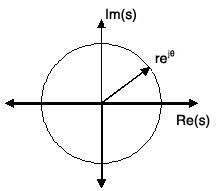
Examples of Pole/Zero Plots
This section lists several examples of finding the poles and zeros of a transfer function and then plotting them onto the S-Plane.
Example 11.6. Simple Pole/Zero Plot
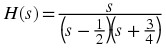
The zeros are: {0}
The poles are:
Figure 11.10. Pole/Zero Plot

Using the zeros and poles found from the transfer function, the one zero is mapped to zero and the two poles are placed atand

Example 11.7. Complex Pole/Zero Plot
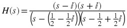
The zeros are: {ⅈ, – ⅈ}
The poles are:
Figure 11.11. Pole/Zero Plot
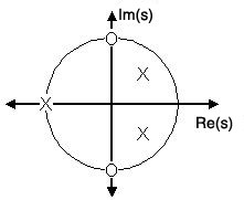
Using the zeros and poles found from the transfer function, the zeros are mapped to ± ⅈ , and the poles are placed at – 1,and

Example 11.8. Pole-Zero Cancellation
An easy mistake to make with regards to poles and zeros is to think that a function likeis the same as s + 3 . In theory they are equivalent, as the pole and zero at s = 1 cancel each other out in what is known as pole-zero cancellation. However, think about what may happen if this were a transfer function of a system that was created with physical circuits. In this case, it is very unlikely that the pole and zero would remain in exactly the same place. A minor temperature change, for instance, could cause one of them to move just slightly. If this were to occur a tremendous amount of volatility is created in that area, since there is a change from infinity at the pole to zero at the zero in a very small range of signals. This is generally a very bad way to try to eliminate a pole. A much better way is to use control theory to move the pole to a better place.
Repeated Poles and Zeros
It is possible to have more than one pole or zero at any given point. For instance, the discrete-time transfer function H(z) = z 2 will have two zeros at the origin and the continuous-time functionwill have 25 poles at the origin.
MATLAB - If access to MATLAB is readily available, then you can use its functions to easily create pole/zero plots. Below is a short program that plots the poles and zeros from the above example onto the Z-Plane.
% Set up vector for zeros
z = [j ; -j];
% Set up vector for poles
p = [-1 ; .5+.5j ; .5-.5j];
figure(1);
zplane(z,p);
title('Pole/Zero Plot for Complex Pole/Zero Plot Example');
Interactive Demonstration of Poles and Zeros
Figure 11.12.
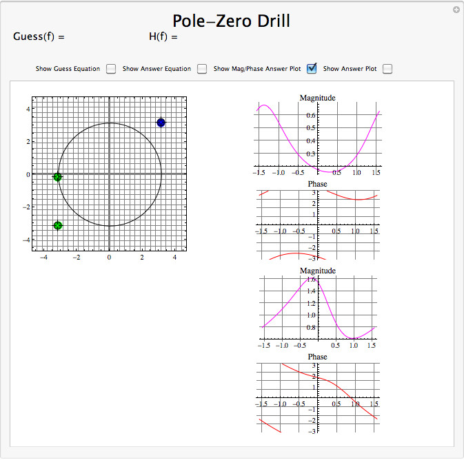
Interact (when online) with a Mathematica CDF demonstrating Pole/Zero Plots. To Download, right-click and save target as .cdf.
Applications for pole-zero plots
Stability and Control theory
Now that we have found and plotted the poles and zeros, we must ask what it is that this plot gives us. Basically what we can gather from this is that the magnitude of the transfer function will be larger when it is closer to the poles and smaller when it is closer to the zeros. This provides us with a qualitative understanding of what the system does at various frequencies and is crucial to the discussion of stability.
Pole/Zero Plots and the Region of Convergence
The region of convergence (ROC) for X(z) in the complex Z-plane can be determined from the pole/zero plot. Although several regions of convergence may be possible, where each one corresponds to a different impulse response, there are some choices that are more practical. A ROC can be chosen to make the transfer function causal and/or stable depending on the pole/zero plot.
Filter Properties from ROC
If the ROC extends outward from the outermost pole, then the system is causal.
If the ROC includes the unit circle, then the system is stable.
Below is a pole/zero plot with a possible ROC of the Z-transform in the Simple Pole/Zero Plot discussed earlier. The shaded region indicates the ROC chosen for the filter. From this figure, we can see that the filter will be both causal and stable since the above listed conditions are both met.
Example 11.9.

Figure 11.13. Region of Convergence for the Pole/Zero Plot
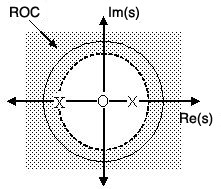
The shaded area represents the chosen ROC for the transfer function.
Frequency Response and Pole/Zero Plots
The reason it is helpful to understand and create these pole/zero plots is due to their ability to help us easily design a filter. Based on the location of the poles and zeros, the magnitude response of the filter can be quickly understood. Also, by starting with the pole/zero plot, one can design a filter and obtain its transfer function very easily.
Conclusion
Pole-Zero Plots are clearly quite useful in the study of the Laplace and Z transform, affording us a method of visualizing the at times confusing mathematical functions.
11.6. Region of Convergence for the Laplace Transform*
Introduction
With the Laplace transform, the s-plane represents a set of signals (complex exponentials). For any given LTI system, some of these signals may cause the output of the system to converge, while others cause the output to diverge ("blow up"). The set of signals that cause the system's output to converge lie in the region of convergence (ROC). This module will discuss how to find this region of convergence for any continuous-time, LTI system.
The Region of Convergence
The region of convergence, known as the ROC, is important to understand because it defines the region where the Laplace transform exists. The Laplace transform of a sequence is defined as 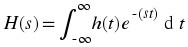 The ROC for a given h(t) , is defined as the range of t for which the Laplace transform converges. If we consider a causal, complex exponential, h(t) = ⅇ
– (at)
u(t) , we get the equation,
The ROC for a given h(t) , is defined as the range of t for which the Laplace transform converges. If we consider a causal, complex exponential, h(t) = ⅇ
– (at)
u(t) , we get the equation, 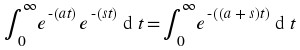 Evaluating this, we get
  Notice that this equation will tend to infinity when
 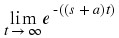 tends to infinity. To understand when this happens, we take one more step by using s = σ + ⅈω to realize this equation as
 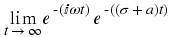 Recognizing that ⅇ
– (ⅈωt) is sinusoidal, it becomes apparent that ⅇ
– (σ(a)t) is going to determine whether this blows up or not. What we find is that if σ + a is positive, the exponential will be to a negative power, which will cause it to go to zero as t tends to infinity. On the other hand, if σ + a is negative or zero, the exponential will not be to a negative power, which will prevent it from tending to zero and the system will not converge. What all of this tells us is that for a causal signal, we have convergence when
Recognizing that ⅇ
– (ⅈωt) is sinusoidal, it becomes apparent that ⅇ
– (σ(a)t) is going to determine whether this blows up or not. What we find is that if σ + a is positive, the exponential will be to a negative power, which will cause it to go to zero as t tends to infinity. On the other hand, if σ + a is negative or zero, the exponential will not be to a negative power, which will prevent it from tending to zero and the system will not converge. What all of this tells us is that for a causal signal, we have convergence when
(11.6)
Condition for Convergence
Re(s) > – a
Alternatively, we can note that since the Laplace transform is a power series, it converges when h(t)ⅇ
– (st) is absolutely summable. Therefore, 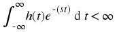 must be satisfied for convergence.
Although we will not go through the process again for anticausal signals, we could. In doing so, we would find that the necessary condition for convergence is when
(11.7)
Necessary Condition for Anti-Causal Convergence
Re(s) < – a
Properties of the Region of Convergencec
The Region of Convergence has a number of properties that are dependent on the characteristics of the signal, h(t) .
The ROC cannot contain any poles. By definition a pole is a where H(s) is infinite. Since H(s) must be finite for all s for convergence, there cannot be a pole in the ROC.
If h(t) is a finite-duration sequence, then the ROC is the entire s-plane, except possibly s = 0 or |s| = ∞ . A finite-duration sequence is a sequence that is nonzero in a finite interval t1 ≤ t ≤ t2 . As long as each value of h(t) is finite then the sequence will be absolutely summable. When t 2 > 0 there will be a s -1 term and thus the ROC will not include s = 0 . When t 1 < 0 then the sum will be infinite and thus the ROC will not include |s| = ∞ . On the other hand, when t 2 ≤ 0 then the ROC will include s = 0 , and when t 1 ≥ 0 the ROC will include |s| = ∞ . With these constraints, the only signal, then, whose ROC is the entire z-plane is h(t) = c δ(t) .
Figure 11.14.
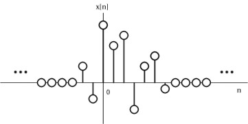
An example of a finite duration sequence.
The next properties apply to infinite duration sequences. As noted above, the z-transform converges when |H(s)| < ∞ . So we can write  We can then split the infinite sum into positive-time and negative-time portions. So |H(s)| ≤ N(s) + P(s) where
 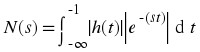 and
and 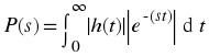 In order for |H(s)| to be finite, |h(t)| must be bounded. Let us then set |h(t)| ≤ C
1
r
1
t
for t < 0 and |h(t)| ≤ C
2
r
2
t
for t ≥ 0 From this some further properties can be derived:
In order for |H(s)| to be finite, |h(t)| must be bounded. Let us then set |h(t)| ≤ C
1
r
1
t
for t < 0 and |h(t)| ≤ C
2
r
2
t
for t ≥ 0 From this some further properties can be derived:
If h(t) is a right-sided sequence, then the ROC extends outward from the outermost pole in H(s) . A right-sided sequence is a sequence where h(t) = 0 for t < t1 < ∞ . Looking at the positive-time portion from the above derivation, it follows that
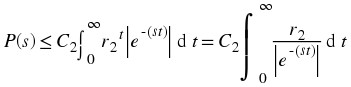 Thus in order for this integral to converge, |ⅇ
– s
| > r
2 , and therefore the ROC of a right-sided sequence is of the form |ⅇ
– s
| > r
2 .
Thus in order for this integral to converge, |ⅇ
– s
| > r
2 , and therefore the ROC of a right-sided sequence is of the form |ⅇ
– s
| > r
2 .
Figure 11.15.
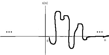
A right-sided sequence.
Figure 11.16.

The ROC of a right-sided sequence.
If h(t) is a left-sided sequence, then the ROC extends inward from the innermost pole in H(s) . A left-sided sequence is a sequence where h(t) = 0 for t > t1 > – ∞ . Looking at the negative-time portion from the above derivation, it follows that
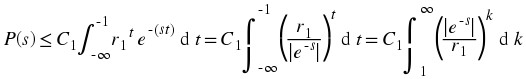 Thus in order for this integral to converge, |ⅇ
– s
| < r
1 , and therefore the ROC of a left-sided sequence is of the form |ⅇ
– s
| < r
1 .
Thus in order for this integral to converge, |ⅇ
– s
| < r
1 , and therefore the ROC of a left-sided sequence is of the form |ⅇ
– s
| < r
1 .
Figure 11.17.
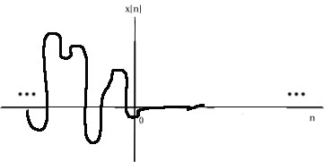
A left-sided sequence.
Figure 11.18.

The ROC of a left-sided sequence.
If h(t) is a two-sided sequence, the ROC will be a ring in the z-plane that is bounded on the interior and exterior by a pole. A two-sided sequence is an sequence with infinite duration in the positive and negative directions. From the derivation of the above two properties, it follows that if r 2 < |ⅇ – s | < r 2 converges, then both the positive-time and negative-time portions converge and thus H(s) converges as well. Therefore the ROC of a two-sided sequence is of the form -r2 < |ⅇ – s | < r 2 .
Figure 11.19.
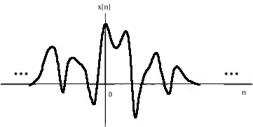
A two-sided sequence.
Figure 11.20.

The ROC of a two-sided sequence.
Examples
To gain further insight it is good to look at a couple of examples.
Example 11.10.
Lets takeThe Laplace-transform of
is
with an ROC at
.
Figure 11.21.

The ROC of

The z-transform ofis
with an ROC at
.
Figure 11.22.

The ROC of

Due to linearity,By observation it is clear that there are two zeros, at 0 and
, and two poles, at
, and
. Following the above properties, the ROC is
.
Figure 11.23.

The ROC of
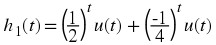
Example 11.11.
Now takeThe z-transform and ROC of
was shown in the example above. The Laplace-transorm of
is
with an ROC at
.
Figure 11.24.
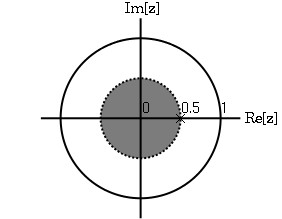
The ROC of
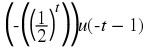
Once again, by linearity,By observation it is again clear that there are two zeros, at 0 and
, and two poles, at
, and
. in ths case though, the ROC is
.
Figure 11.25.

The ROC of.
Graphical Understanding of ROC
Using the demonstration, learn about the region of convergence for the Laplace Transform.
Conclusion
Clearly, in order to craft a system that is actually useful by virtue of being causal and BIBO stable, we must ensure that it is within the Region of Convergence, which can be ascertained by looking at the pole zero plot. The Region of Convergence is the area in the pole/zero plot of the transfer function in which the function exists. For purposes of useful filter design, we prefer to work with rational functions, which can be described by two polynomials, one each for determining the poles and the zeros, respectively.
11.7. Rational Functions and the Laplace Transform*
Introduction
When dealing with operations on polynomials, the term rational function is a simple way to describe a particular relationship between two polynomials.
Definition: rational function
For any two polynomials, A and B, their quotient is called a rational function.
Example .
Below is a simple example of a basic rational function, f(x) . Note that the numerator and denominator can be polynomials of any order, but the rational function is undefined when the denominator equals zero.
Properties of Rational Functions
In order to see what makes rational functions special, let us look at some of their basic properties and characteristics. If you are familiar with rational functions and basic algebraic properties, skip to the next section to see how rational functions are useful when dealing with the Laplace transform.
Roots
To understand many of the following characteristics of a rational function, one must begin by finding the roots of the rational function. In order to do this, let us factor both of the polynomials so that the roots can be easily determined. Like all polynomials, the roots will provide us with information on many key properties. The function below shows the results of factoring the above rational function, Equation.
(11.8)

Thus, the roots of the rational function are as follows:
Roots of the numerator are: {-2, 2}
Roots of the denominator are: {-3, 1}
Note
In order to understand rational functions, it is essential to know and understand the roots that make up the rational function.
Discontinuities
Because we are dealing with division of two polynomials, we must be aware of the values of the variable that will cause the denominator of our fraction to be zero. When this happens, the rational function becomes undefined, i.e. we have a discontinuity in the function. Because we have already solved for our roots, it is very easy to see when this occurs. When the variable in the denominator equals any of the roots of the denominator, the function becomes undefined.
Example 11.13.
Continuing to look at our rational function above, Equation, we can see that the function will have discontinuities at the following points:
In respect to the Cartesian plane, we say that the discontinuities are the values along the x-axis where the function is undefined. These discontinuities often appear as vertical asymptotes on the graph to represent the values where the function is undefined.
Domain
Using the roots that we found above, the domain of the rational function can be easily defined.
Definition: domain
The group, or set, of values that are defined by a given function.
Example .
Using the rational function above, Equation, the domain can be defined as any real number x where x does not equal 1 or negative 3. Written out mathematically, we get the following:

Intercepts
The x-intercept is defined as the point(s) where f(x) , i.e. the output of the rational functions, equals zero. Because we have already found the roots of the equation this process is very simple. From algebra, we know that the output will be zero whenever the numerator of the rational function is equal to zero. Therefore, the function will have an x-intercept wherever x equals one of the roots of the numerator.
The y-intercept occurs whenever x equals zero. This can be found by setting all the values of x equal to zero and solving the rational function.
Rational Functions and the Laplace Transform
Rational functions often result when the Laplace transform is used to compute transfer functions for LTI systems. When using the Laplace transform to solve linear constant coefficient ordinary differential equations, partial fraction expansions of rational functions prove particularly useful. The roots of the polynomials in the numerator and denominator of the transfer function play an important role in describing system behavior. The roots of the polynomial in the numerator produce zeros of the transfer function where the system produces no output for an input of that complex frequency. The roots of the polynomial in the denominator produce poles of the transfer function where the system has natural frequencies of oscillation.
Summary
Once we have used our knowledge of rational functions to find its roots, we can manipulate a Laplace transform in a number of useful ways. We can apply this knowledge by representing an LTI system graphically through a pole-zero plot for analysis or design.
11.8. Differential Equations*
Differential Equations
It is often useful to describe systems using equations involving the rate of change in some quantity through differential equations. Recall that one important subclass of differential equations, linear constant coefficient ordinary differential equations, takes the form
(11.9)A y ( t ) = x ( t )
where A is a differential operator of the form
(11.10)
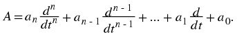
The differential equation in Equation 11.9 would describe some system modeled by A with an input forcing function x(t) that produces an output solution signal y(t). However, the unilateral Laplace transform permits a solution for initial value problems to be found in what is usually a much simpler method. Specifically, it greatly simplifies the procedure for nonhomogeneous differential equations.
General Formulas for the Differential Equation
As stated briefly in the definition above, a differential equation is a very useful tool in describing and calculating the change in an output of a system described by the formula for a given input. The key property of the differential equation is its ability to help easily find the transform, H(s) , of a system. In the following two subsections, we will look at the general form of the differential equation and the general conversion to a Laplace-transform directly from the differential equation.
Conversion to Laplace-Transform
Using the definition, ???, we can easily generalize the transfer function, H(s) , for any differential equation. Below are the steps taken to convert any differential equation into its transfer function, i.e. Laplace-transform. The first step involves taking the Fourier Transform of all the terms in ???. Then we use the linearity property to pull the transform inside the summation and the time-shifting property of the Laplace-transform to change the time-shifting terms to exponentials. Once this is done, we arrive at the following equation: a
0 = 1 . 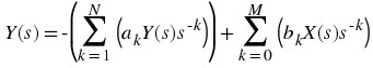

Conversion to Frequency Response
Once the Laplace-transform has been calculated from the differential equation, we can go one step further to define the frequency response of the system, or filter, that is being represented by the differential equation.
Note
Remember that the reason we are dealing with these formulas is to be able to aid us in filter design. A LCCDE is one of the easiest ways to represent FIR filters. By being able to find the frequency response, we will be able to look at the basic properties of any filter represented by a simple LCCDE.
Below is the general formula for the frequency response of a Laplace-transform. The conversion is simply a matter of taking the Laplace-transform formula, H(s) , and replacing every instance of s with ⅇ
ⅈw
. 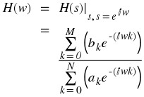 Once you understand the derivation of this formula, look at the module concerning Filter Design from the Laplace-Transform for a look into how all of these ideas of the Laplace-transform, Differential Equation, and Pole/Zero Plots play a role in filter design.
Solving a LCCDE
In order for a linear constant-coefficient difference equation to be useful in analyzing a LTI system, we must be able to find the systems output based upon a known input, x(t) , and a set of initial conditions. Two common methods exist for solving a LCCDE: the direct method and the indirect method, the latter being based on the Laplace-transform. Below we will briefly discuss the formulas for solving a LCCDE using each of these methods.
Direct Method
The final solution to the output based on the direct method is the sum of two parts, expressed in the following equation: y(t) = y h (t) + y p (t) The first part, y h (t) , is referred to as the homogeneous solution and the second part, y h (t) , is referred to as particular solution. The following method is very similar to that used to solve many differential equations, so if you have taken a differential calculus course or used differential equations before then this should seem very familiar.
Homogeneous Solution
We begin by assuming that the input is zero, x(t) = 0 . Now we simply need to solve the homogeneous differential equation: 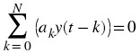 In order to solve this, we will make the assumption that the solution is in the form of an exponential. We will use lambda, λ , to represent our exponential terms. We now have to solve the following equation:
 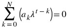 We can expand this equation out and factor out all of the lambda terms. This will give us a large polynomial in parenthesis, which is referred to as the characteristic polynomial. The roots of this polynomial will be the key to solving the homogeneous equation. If there are all distinct roots, then the general solution to the equation will be as follows: y
h
(t) = C
1(λ
1)t
+ C
2(λ
2)t
+ … + C
N
(λ
N
)t
However, if the characteristic equation contains multiple roots then the above general solution will be slightly different. Below we have the modified version for an equation where λ
1
has K multiple roots: y
h
(t) = C
1(λ
1)t
+ C
1
t(λ
1)t
+ C
1
t
2(λ
1)t
+ … + C
1
t
K − 1(λ
1)t
+ C
2(λ
2)t
+ … + C
N
(λ
N
)t
We can expand this equation out and factor out all of the lambda terms. This will give us a large polynomial in parenthesis, which is referred to as the characteristic polynomial. The roots of this polynomial will be the key to solving the homogeneous equation. If there are all distinct roots, then the general solution to the equation will be as follows: y
h
(t) = C
1(λ
1)t
+ C
2(λ
2)t
+ … + C
N
(λ
N
)t
However, if the characteristic equation contains multiple roots then the above general solution will be slightly different. Below we have the modified version for an equation where λ
1
has K multiple roots: y
h
(t) = C
1(λ
1)t
+ C
1
t(λ
1)t
+ C
1
t
2(λ
1)t
+ … + C
1
t
K − 1(λ
1)t
+ C
2(λ
2)t
+ … + C
N
(λ
N
)t
Particular Solution
The particular solution, y
p
(t) , will be any solution that will solve the general differential equation: 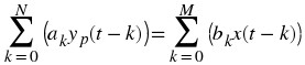 In order to solve, our guess for the solution to y
p
(t) will take on the form of the input, x(t) . After guessing at a solution to the above equation involving the particular solution, one only needs to plug the solution into the differential equation and solve it out.
In order to solve, our guess for the solution to y
p
(t) will take on the form of the input, x(t) . After guessing at a solution to the above equation involving the particular solution, one only needs to plug the solution into the differential equation and solve it out.
Indirect Method
The indirect method utilizes the relationship between the differential equation and the Laplace-transform, discussed earlier, to find a solution. The basic idea is to convert the differential equation into a Laplace-transform, as described above, to get the resulting output, Y(s) . Then by inverse transforming this and using partial-fraction expansion, we can arrive at the solution.
(11.11)
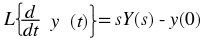
This can be interatively extended to an arbitrary order derivative as in Equation Equation 11.12.
(11.12)

Now, the Laplace transform of each side of the differential equation can be taken
(11.13)
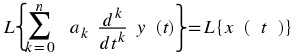
which by linearity results in
(11.14)
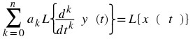
and by differentiation properties in
(11.15)
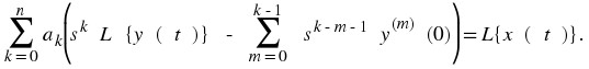
Rearranging terms to isolate the Laplace transform of the output,
(11.16)
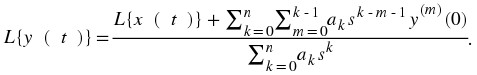
Thus, it is found that
(11.17)
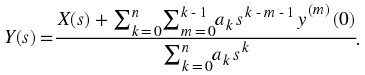
In order to find the output, it only remains to find the Laplace transform X(s) of the input, substitute the initial conditions, and compute the inverse Laplace transform of the result. Partial fraction expansions are often required for this last step. This may sound daunting while looking at Equation Equation 11.17, but it is often easy in practice, especially for low order differential equations. Equation Equation 11.17 can also be used to determine the transfer function and frequency response.
As an example, consider the differential equation
(11.18)
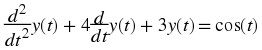
with the initial conditions y ' (0) = 1 and y(0) = 0 Using the method described above, the Laplace transform of the solution y(t) is given by
(11.19)
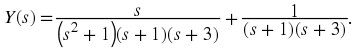
Performing a partial fraction decomposition, this also equals
(11.20)
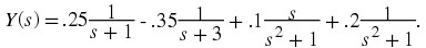
Computing the inverse Laplace transform,
(11.21)

One can check that this satisfies that this satisfies both the differential equation and the initial conditions.
Summary
One of the most important concepts of DSP is to be able to properly represent the input/output relationship to a given LTI system. A linear constant-coefficient difference equation (LCCDE) serves as a way to express just this relationship in a discrete-time system. Writing the sequence of inputs and outputs, which represent the characteristics of the LTI system, as a difference equation helps in understanding and manipulating a system.
11.9. Continuous Time Filter Design*
Introduction
Analog (Continuous-Time) filters are useful for a wide variety of applications, and are especially useful in that they are very simple to build using standard, passive R,L,C components. Having a grounding in basic filter design theory can assist one in solving a wide variety of signal processing problems.
Estimating Frequency Response from Z-Plane
One of the motivating factors for analyzing the pole/zero plots is due to their relationship to the frequency response of the system. Based on the position of the poles and zeros, one can quickly determine the frequency response. This is a result of the correspondence between the frequency response and the transfer function evaluated on the unit circle in the pole/zero plots. The frequency response, or DTFT, of the system is defined as:  Next, by factoring the transfer function into poles and zeros and multiplying the numerator and denominator by ⅇ
ⅈw
we arrive at the following equations:
Next, by factoring the transfer function into poles and zeros and multiplying the numerator and denominator by ⅇ
ⅈw
we arrive at the following equations: 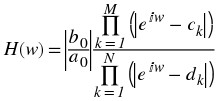 From Equation we have the frequency response in a form that can be used to interpret physical characteristics about the filter's frequency response. The numerator and denominator contain a product of terms of the form |ⅇ
ⅈw
− h|, where h is either a zero, denoted by c
k
or a pole, denoted by d
k
. Vectors are commonly used to represent the term and its parts on the complex plane. The pole or zero, h , is a vector from the origin to its location anywhere on the complex plane and ⅇ
ⅈw
is a vector from the origin to its location on the unit circle. The vector connecting these two points, |ⅇ
ⅈw
− h|, connects the pole or zero location to a place on the unit circle dependent on the value of w . From this, we can begin to understand how the magnitude of the frequency response is a ratio of the distances to the poles and zero present in the z-plane as w goes from zero to pi. These characteristics allow us to interpret |H(w)| as follows:
From Equation we have the frequency response in a form that can be used to interpret physical characteristics about the filter's frequency response. The numerator and denominator contain a product of terms of the form |ⅇ
ⅈw
− h|, where h is either a zero, denoted by c
k
or a pole, denoted by d
k
. Vectors are commonly used to represent the term and its parts on the complex plane. The pole or zero, h , is a vector from the origin to its location anywhere on the complex plane and ⅇ
ⅈw
is a vector from the origin to its location on the unit circle. The vector connecting these two points, |ⅇ
ⅈw
− h|, connects the pole or zero location to a place on the unit circle dependent on the value of w . From this, we can begin to understand how the magnitude of the frequency response is a ratio of the distances to the poles and zero present in the z-plane as w goes from zero to pi. These characteristics allow us to interpret |H(w)| as follows:  In conclusion, using the distances from the unit circle to the poles and zeros, we can plot the frequency response of the system. As w goes from 0 to 2π , the following two properties, taken from the above equations, specify how one should draw |H(w)|.
While moving around the unit circle...
if close to a zero, then the magnitude is small. If a zero is on the unit circle, then the frequency response is zero at that point.
if close to a pole, then the magnitude is large. If a pole is on the unit circle, then the frequency response goes to infinity at that point.
Drawing Frequency Response from Pole/Zero Plot
Let us now look at several examples of determining the magnitude of the frequency response from the pole/zero plot of a z-transform. If you have forgotten or are unfamiliar with pole/zero plots, please refer back to the Pole/Zero Plots module.
Example 11.15.
In this first example we will take a look at the very simple z-transform shown below: H(z) = z + 1 = 1 + z -1 H(w) = 1 + ⅇ – (ⅈw) For this example, some of the vectors represented by |ⅇ ⅈw − h|, for random values of w , are explicitly drawn onto the complex plane shown in the figure below. These vectors show how the amplitude of the frequency response changes as w goes from 0 to 2π , and also show the physical meaning of the terms in Equation above. One can see that when w = 0, the vector is the longest and thus the frequency response will have its largest amplitude here. As w approaches π , the length of the vectors decrease as does the amplitude of |H(w)|. Since there are no poles in the transform, there is only this one vector term rather than a ratio as seen in Equation.
Figure 11.26. Pole/Zero Plot
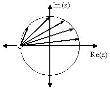
(a)

(b)
The first figure represents the pole/zero plot with a few representative vectors graphed while the second shows the frequency response with a peak at +2 and graphed between plus and minus π .
Example 11.16.
For this example, a more complex transfer function is analyzed in order to represent the system's frequency response.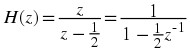

Below we can see the two figures described by the above equations. The Figure 11.27 represents the basic pole/zero plot of the z-transform, H(w). Figure 11.27 shows the magnitude of the frequency response. From the formulas and statements in the previous section, we can see that when w = 0 the frequency will peak since it is at this value of w that the pole is closest to the unit circle. The ratio from Equation helps us see the mathematics behind this conclusion and the relationship between the distances from the unit circle and the poles and zeros. As w moves from 0 to π , we see how the zero begins to mask the effects of the pole and thus force the frequency response closer to 0.
Figure 11.27. Pole/Zero Plot

(a)

(b)
The first figure represents the pole/zero plot while the second shows the frequency response with a peak at +2 and graphed between plus and minus π .
Types of Filters
Butterworth Filters
The Butterworth filter is the simplest filter. It can be constructed out of passive R, L, C circuits. The magnitude of the transfer function for this filter is
(11.22)
Magnitude of Butterworth Filter Transfer Function
where n is the order of the filter and ω
c
is the cutoff frequency. The cutoff frequency is the frequency where the magnitude experiences a 3 dB dropoff (where  ).
).
Figure 11.28.
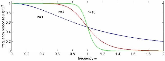
Three different orders of lowpass Butterworth analog filters: n = {1, 4, 10} . As n increases, the filter more closely approximates an ideal brickwall lowpass response.
The important aspects of Figure 11.28 are that it does not ripple in the passband or stopband as other filters tend to, and that the larger n , the sharper the cutoff (the smaller the transition band).
Butterworth filters give transfer functions (H(ⅈω) and H(s) ) that are rational functions. They also have only poles, resulting in a transfer function of the form 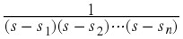 and a pole-zero plot of
Figure 11.29.

Poles of a 10th-order ( n = 5 ) lowpass Butterworth filter.
Note that the poles lie along a circle in the s-plane.
Chebyshev Filters
The Butterworth filter does not give a sufficiently good approximation across the complete passband in many cases. The Taylor's series approximation is often not suited to the way specifications are given for filters. An alternate error measure is the maximum of the absolute value of the difference between the actual filter response and the ideal. This is considered over the total passband. This is the Chebyshev error measure and was defined and applied to the FIR filter design problem. For the IIR filter, the Chebyshev error is minimized over the passband and a Taylor's series approximation at ω = ∞ is used to determine the stopband performance. This mixture of methods in the IIR case is called the Chebyshev filter, and simple design formulas result, just as for the Butterworth filter.
The design of Chebyshev filters is particularly interesting, because the results of a very elegant theory insure that constructing a frequency-response function with the proper form of equal ripple in the error will result in a minimum Chebyshev error without explicitly minimizing anything. This allows a straightforward set of design formulas to be derived which can be viewed as a generalization of the Butterworth formulas ???, ???.
The form for the magnitude squared of the frequency-response function for the Chebyshev filter is
(11.23)
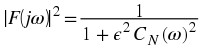
where C N (ω) is an Nth-order Chebyshev polynomial and ϵ is a parameter that controls the ripple size. This polynomial in ω has very special characteristics that result in the optimality of the response function (Equation 11.23).
Figure 11.30.
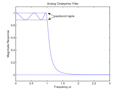
Fifth Order Chebyshev Filter Frequency Response
Bessel filters
Insert bessel filter information
Elliptic Filters
There is yet another method that has been developed that uses a Chebyshev error criterion in both the passband and the stopband. This is the fourth possible combination of Chebyshev and Taylor's series approximations in the passband and stopband. The resulting filter is called an elliptic-function filter, because elliptic functions are normally used to calculate the pole and zero locations. It is also sometimes called a Cauer filter or a rational Chebyshev filter, and it has equal ripple approximation error in both pass and stopbands ???, ???, ???, ???.
The error criteria of the elliptic-function filter are particularly well suited to the way specifications for filters are often given. For that reason, use of the elliptic-function filter design usually gives the lowest order filter of the four classical filter design methods for a given set of specifications. Unfortunately, the design of this filter is the most complicated of the four. However, because of the efficiency of this class of filters, it is worthwhile gaining some understanding of the mathematics behind the design procedure.
This section sketches an outline of the theory of elliptic- function filter design. The details and properties of the elliptic functions themselves should simply be accepted, and attention put on understanding the overall picture. A more complete development is available in ???, ???.
Because both the passband and stopband approximations are over the entire bands, a transition band between the two must be defined. Using a normalized passband edge, the bands are defined by
(11.24)
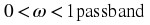
(11.25)
(11.26)
This is illustrated in Figure .
Figure 11.31.
Third Order Analog Elliptic Function Lowpass Filter showing the Ripples and Band Edges
The characteristics of the elliptic function filter are best described in terms of the four parameters that specify the frequency response:
The maximum variation or ripple in the passband δ 1 ,
The width of the transition band
 ,
, The maximum response or ripple in the stopband δ 2 , and
The order of the filter N .
The result of the design is that for any three of the parameters given, the fourth is minimum. This is a very flexible and powerful description of a filter frequency response.
The form of the frequency-response function is a generalization of that for the Chebyshev filter
(11.27)
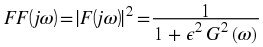
where
(11.28)F F ( s ) = F ( s ) F ( – s )
with F(s) being the prototype analog filter transfer function similar to that for the Chebyshev filter. G(ω) is a rational function that approximates zero in the passband and infinity in the stopband. The definition of this function is a generalization of the definition of the Chebyshev polynomial.
Filter Design Demonstration
Conclusion
As can be seen, there is a large amount of information available in filter design, more than an introductory module can cover. Even for designing Discrete-time IIR filters, it is important to remember that there is a far larger body of literature for design methods for the analog signal processing world than there is for the digital. Therefore, it is often easier and more practical to implement an IIR filter using standard analog methods, and then discretize it using methods such as the Bilateral Transform.
Chapter 12. Z-Transform and Discrete Time System Design
12.1. Z-Transform*
Introduction
The Z transform is a generalization of the Discrete-Time Fourier Transform. It is used because the DTFT does not converge/exist for many important signals, and yet does for the z-transform. It is also used because it is notationally cleaner than the DTFT. In contrast to the DTFT, instead of using complex exponentials of the form ⅇ ⅈωn , with purely imaginary parameters, the Z transform uses the more general, z n , where z is complex. The Z-transform thus allows one to bring in the power of complex variable theory into Digital Signal Processing.
The Z-Transform
Bilateral Z-transform Pair
Although Z transforms are rarely solved in practice using integration (tables and computers (e.g. Matlab) are much more common), we will provide the bilateral Z transform pair here for purposes of discussion and derivation. These define the forward and inverse Z transformations. Notice the similarities between the forward and inverse transforms. This will give rise to many of the same symmetries found in Fourier analysis.
(12.1)
Z Transform

(12.2)
Inverse Z Transform

Note
We have defined the bilateral z-transform. There is also a unilateral z-transform ,
(12.3)
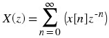
which is useful for solving the difference equations with nonzero initial conditions. This is similar to the unilateral Laplace Transform in continuous time.
Relation between Z-transform and DTFT
Taking a look at the equations describing the Z-Transform and the Discrete-Time Fourier Transform:
(12.4)
Discrete-Time Fourier Transform
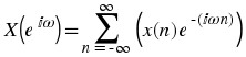
(12.5)
Z-Transform

We can see many similarities; first, that : X(ⅇ ⅈω ) = X(z) for all z = ⅇ ⅈω
Visualizing the Z-transform
With the DTFT, we have a complex-valued function of a real-valued variable ω (and 2 π periodic). The Z-transform is a complex-valued function of a complex valued variable z.
Figure 12.1. Plots
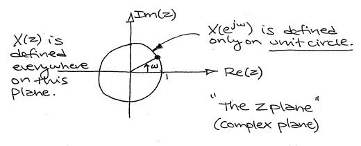
With the Fourier transform, we had a complex-valued function of a purely imaginary variable, F(ⅈω) . This was something we could envision with two 2-dimensional plots (real and imaginary parts or magnitude and phase). However, with Z, we have a complex-valued function of a complex variable. In order to examine the magnitude and phase or real and imaginary parts of this function, we must examine 3-dimensional surface plots of each component.
Consider the z-transform given by H(z) = z , as illustrated below.
Figure 12.2.
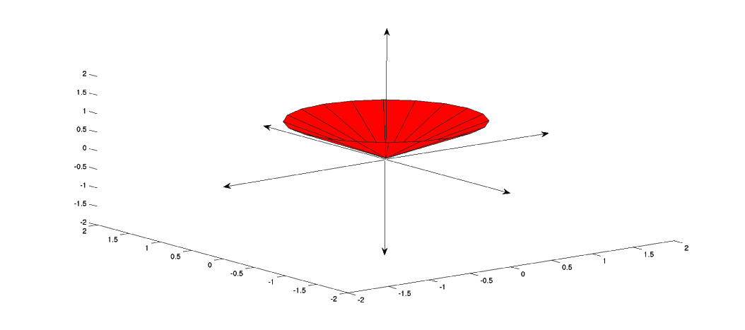
The corresponding DTFT has magnitude and phase given below.
Note
While these are legitimate ways of looking at a signal in the Z domain, it is quite difficult to draw and/or analyze. For this reason, a simpler method has been developed. Although it will not be discussed in detail here, the method of Poles and Zeros is much easier to understand and is the way both the Z transform and its continuous-time counterpart the Laplace-transform are represented graphically.
Figure 12.3.
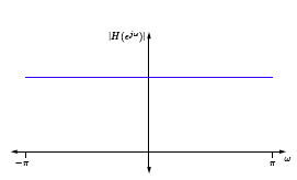
(a)
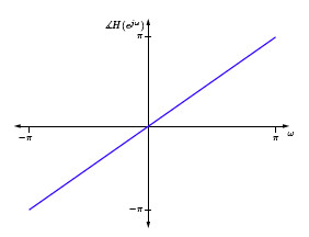
(b)
Magnitude and Phase of H(z).
What could the system H be doing? It is a perfect all-pass, linear-phase system. But what does this mean?
Suppose 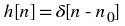 . Then
(12.6)
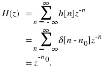
Thus, H(z) = z – n 0 is the z -transform of a system that simply delays the input by n 0 . H(z) is the z -transform of a unit-delay.
Now consider x[n] = α n u[n]
Figure 12.4.
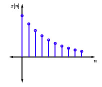
(12.7)

What if  ? Then
  does not converge! Therefore, whenever we compute a z -tranform, we must also specify the set of z 's for which the z -transform exists. This is called the regionofconvergence (ROC).
Using a computer to find the Z-Transform
Matlab has two functions, ztrans and iztrans, that are both part of the symbolic toolbox, and will find the Z and inverse Z transforms respectively. This method is generally preferred for more complicated functions. Simpler and more contrived functions are usually found easily enough by using tables.
Application to Discrete Time Filters
The z -transform might seem slightly ugly. We have to worry about the region of convergence, and stability issues, and so forth. However, in the end it is worthwhile because it proves extremely useful in analyzing digital filters with feedback. For example, consider the system illustrated below
Figure 12.5. Plots
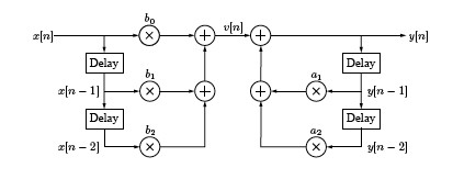
We can analyze this system via the equations
(12.8)

and
(12.9)

More generally,
(12.10)
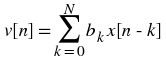
and
(12.11)
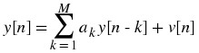
or equivalently,
(12.12)
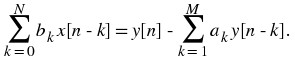
What does the z -transform of this relationship look like?
(12.13)
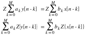
Note that
(12.14)
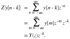
Thus the relationship reduces to
(12.15)
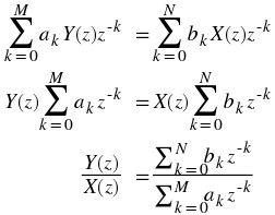
Hence, given a system the one above, we can easily determine the system's transfer function, and end up with a ratio of two polynomials in z : a rational function. Similarly, given a rational function, it is easy to realize this function in a simple hardware architecture.
Interactive Z-Transform Demonstration
Figure 12.6.
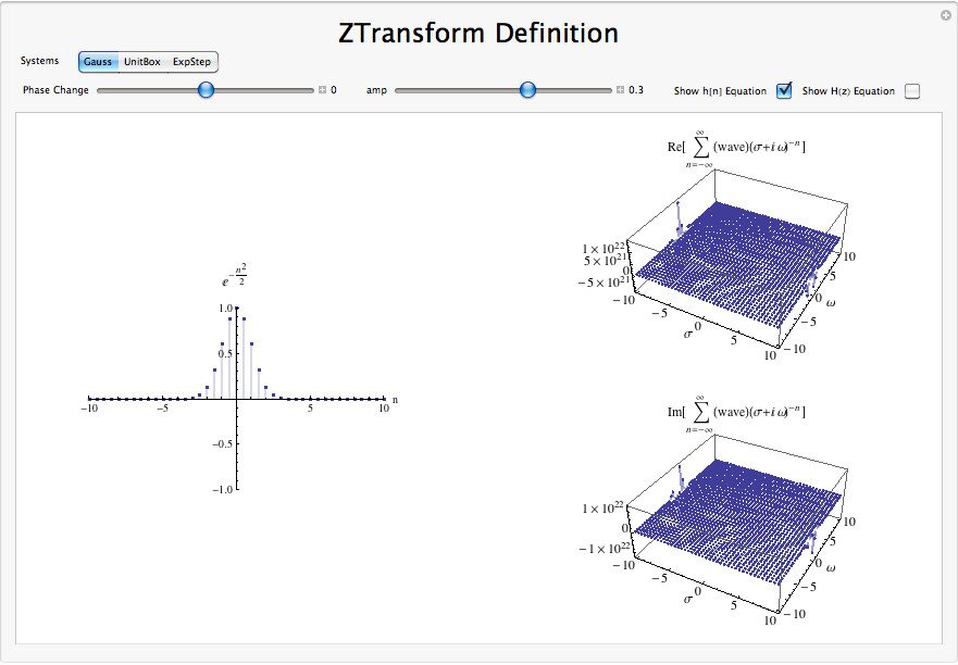
Interact (when online) with a Mathematica CDF demonstrating the Z Transform. To Download, right-click and save target as .cdf.
Conclusion
The z-transform proves a useful, more general form of the Discrete Time Fourier Transform. It applies equally well to describing systems as well as signals using the eigenfunction method, and proves extremely useful in digital filter design.
12.2. Common Z-Transforms*
| Signal | Z-transform | Region of Convergence |
|---|---|---|
| δ ( t ) | 1 | all s |
| δ ( t – T ) | e – ( s T ) | all s |
| u ( t ) | 
| R > 0 |
| – u ( – t ) | 
| R < 0 |
| t u ( t ) | 
| R > 0 |
| t n u ( t ) | 
| R > 0 |

| 
| R < 0 |
| e – ( λ t ) u ( t ) | 
| R > – λ |
| 
| R < – λ |
| t e – ( λ t ) u ( t ) | 
| R > – λ |
| t n e – ( λ t ) u ( t ) | 
| R > – λ |
| 
| R < – λ |
| cos ( b t ) u ( t ) | 
| R > 0 |
| sin ( b t ) u ( t ) | 
| R > 0 |
| e – ( a t ) cos ( b t ) u ( t ) | 
| R > – a |
| e – ( a t ) sin ( b t ) u ( t ) | 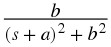
| R > – a |

| s n | all s |
12.3. Properties of the Z-Transform*
Introduction
This module will look at some of the basic properties of the Z-Transform (DTFT).
Note
We will be discussing these properties for aperiodic, discrete-time signals but understand that very similar properties hold for continuous-time signals and periodic signals as well.
Discussion of Z-Transform Properties
Linearity
The combined addition and scalar multiplication properties in the table above demonstrate the basic property of linearity. What you should see is that if one takes the Z-transform of a linear combination of signals then it will be the same as the linear combination of the Z-transforms of each of the individual signals. This is crucial when using a table of transforms to find the transform of a more complicated signal.
Example 12.1.
We will begin with the following signal: x[n] = a f 1[n] + b f 2[n] Now, after we take the Fourier transform, shown in the equation below, notice that the linear combination of the terms is unaffected by the transform. X(z) = a F 1(z) + b F 2(z)
Symmetry
Symmetry is a property that can make life quite easy when solving problems involving Z-transforms. Basically what this property says is that since a rectangular function in time is a sinc function in frequency, then a sinc function in time will be a rectangular function in frequency. This is a direct result of the symmetry between the forward Z and the inverse Z transform. The only difference is the scaling by 2π and a frequency reversal.
Time Scaling
This property deals with the effect on the frequency-domain representation of a signal if the time variable is altered. The most important concept to understand for the time scaling property is that signals that are narrow in time will be broad in frequency and vice versa. The simplest example of this is a delta function, a unit pulse with a very small duration, in time that becomes an infinite-length constant function in frequency.
The table above shows this idea for the general transformation from the time-domain to the frequency-domain of a signal. You should be able to easily notice that these equations show the relationship mentioned previously: if the time variable is increased then the frequency range will be decreased.
Time Shifting
Time shifting shows that a shift in time is equivalent to a linear phase shift in frequency. Since the frequency content depends only on the shape of a signal, which is unchanged in a time shift, then only the phase spectrum will be altered. This property is proven below:
Example 12.2.
We will begin by letting x[n] = f[n − η] . Now let's take the z-transform with the previous expression substituted in for x[n] .Now let's make a simple change of variables, where σ = n − η . Through the calculations below, you can see that only the variable in the exponential are altered thus only changing the phase in the frequency domain.
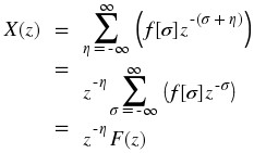
Convolution
Convolution is one of the big reasons for converting signals to the frequency domain, since convolution in time becomes multiplication in frequency. This property is also another excellent example of symmetry between time and frequency. It also shows that there may be little to gain by changing to the frequency domain when multiplication in time is involved.
We will introduce the convolution integral here, but if you have not seen this before or need to refresh your memory, then look at the discrete-time convolution module for a more in depth explanation and derivation.
(12.16)

Time Differentiation
Since discrete LTI systems can be represented in terms of difference equations, it is apparent with this property that converting to the frequency domain may allow us to convert these complicated difference equations to simpler equations involving multiplication and addition.
Parseval's Relation
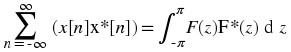 Parseval's relation tells us that the energy of a signal is equal to the energy of its Fourier transform.
Figure 12.7.

Modulation (Frequency Shift)
Modulation is absolutely imperative to communications applications. Being able to shift a signal to a different frequency, allows us to take advantage of different parts of the electromagnetic spectrum is what allows us to transmit television, radio and other applications through the same space without significant interference.
The proof of the frequency shift property is very similar to that of the time shift; however, here we would use the inverse Fourier transform in place of the Fourier transform. Since we went through the steps in the previous, time-shift proof, below we will just show the initial and final step to this proof:  Now we would simply reduce this equation through another change of variables and simplify the terms. Then we will prove the property expressed in the table above: z(t) = f(t)ⅇ
ⅈφt
Now we would simply reduce this equation through another change of variables and simplify the terms. Then we will prove the property expressed in the table above: z(t) = f(t)ⅇ
ⅈφt
Properties Demonstration
An interactive example demonstration of the properties is included below:
Figure 12.8.
(This media type is not supported in this reader. Click to open media in browser.)
Interactive Signal Processing Laboratory Virtual Instrument created using NI's Labview.
Summary Table
| Property | Signal | Z-Transform | Region of Convergence |
| Linearity | α x 1 ( n ) + β x 2 ( n ) | α X 1 ( z ) + β X 2 ( z ) | At least ROC 1∩ ROC 2 |
| Time shifing | x ( n – k ) | z – k X ( z ) | ROC |
| Time scaling | x ( n / k ) | 
| ROC 1 / k |
| Z-domain scaling | a n x ( n ) | X ( z / a ) | | a | ROC |
| Conjugation | 
| 
| ROC |
| Convolution | x 1 ( n ) * x 2 ( n ) | X 1 ( z ) X 2 ( z ) | At least ROC 1∩ ROC 2 |
| Differentiation in z-Domain | [ n x [ n ] ] | 
| ROC= all R |
| Parseval's Theorem | 
| 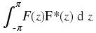
| ROC |
12.4. Inverse Z-Transform*
Introduction
When using the z-transform
 it is often useful to be able to find x[n] given X(z) . There are at least 4 different methods to do this:
Inspection Method
This "method" is to basically become familiar with the z-transform pair tables and then "reverse engineer".
Example 12.3.
When givenwith an ROC of |z| > α we could determine "by inspection" that x[n] = α n u[n]
Partial-Fraction Expansion Method
When dealing with linear time-invariant systems the z-transform is often of the form  This can also expressed as
 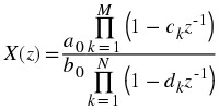 where c
k
represents the nonzero zeros of X(z) and d
k
represents the nonzero poles.
where c
k
represents the nonzero zeros of X(z) and d
k
represents the nonzero poles.
If M < N then X(z) can be represented as 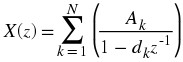 This form allows for easy inversions of each term of the sum using the inspection method and the transform table. If the numerator is a polynomial, however, then it becomes necessary to use partial-fraction expansion to put X(z) in the above form. If M ≥ N then X(z) can be expressed as
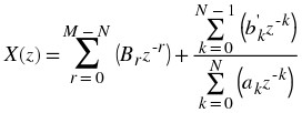
Example 12.4.
Find the inverse z-transform ofwhere the ROC is |z| > 2 . In this case M = N = 2 , so we have to use long division to get
Next factor the denominator.
Now do partial-fraction expansion.
Now each term can be inverted using the inspection method and the z-transform table. Thus, since the ROC is |z| > 2 ,
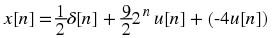
Demonstration of Partial Fraction Expansion
Figure 12.9.
(This media type is not supported in this reader. Click to open media in browser.)
Interactive experiment illustrating how the Partial Fraction Expansion method is used to solve a variety of numerator and denominator problems. (To view and interact with the simulation, download the free Mathematica player at http://www.wolfram.com/products/player/download.cgi)
Figure 12.10. Khan Lecture on Partial Fraction Expansion
(This media type is not supported in this reader. Click to open media in browser.)
video from Khan Academy
Power Series Expansion Method
When the z-transform is defined as a power series in the form  then each term of the sequence x[n] can be determined by looking at the coefficients of the respective power of z
– n
.
then each term of the sequence x[n] can be determined by looking at the coefficients of the respective power of z
– n
.
Example 12.5.
Now look at the z-transform of a finite-length sequence.In this case, since there were no poles, we multiplied the factors of X(z) . Now, by inspection, it is clear that
.
One of the advantages of the power series expansion method is that many functions encountered in engineering problems have their power series' tabulated. Thus functions such as log, sin, exponent, sinh, etc, can be easily inverted.
Example 12.6.
Suppose X(z) = logn (1 + α z -1) Noting thatThen
Therefore

Contour Integration Method
Without going in to much detail 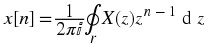 where r is a counter-clockwise contour in the ROC of X(z) encircling the origin of the z-plane. To further expand on this method of finding the inverse requires the knowledge of complex variable theory and thus will not be addressed in this module.
Demonstration of Contour Integration
Figure 12.11.
(This media type is not supported in this reader. Click to open media in browser.)
Interactive experiment illustrating how the contour integral is applied on a simple example. For a more in-depth discussion of this method, some background in complex analysis is required. (To view and interact with the simulation, download the free Mathematica player at http://www.wolfram.com/products/player/download.cgi)
Conclusion
The Inverse Z-transform is very useful to know for the purposes of designing a filter, and there are many ways in which to calculate it, drawing from many disparate areas of mathematics. All nevertheless assist the user in reaching the desired time-domain signal that can then be synthesized in hardware(or software) for implementation in a real-world filter.
12.5. Poles and Zeros in the Z-Plane*
Introduction to Poles and Zeros of the Z-Transform
It is quite difficult to qualitatively analyze the Laplace transform and Z-transform, since mappings of their magnitude and phase or real part and imaginary part result in multiple mappings of 2-dimensional surfaces in 3-dimensional space. For this reason, it is very common to examine a plot of a transfer function's poles and zeros to try to gain a qualitative idea of what a system does.
Once the Z-transform of a system has been determined, one can use the information contained in function's polynomials to graphically represent the function and easily observe many defining characteristics. The Z-transform will have the below structure, based on Rational Functions: 
The two polynomials, P(z) and Q(z), allow us to find the poles and zeros of the Z-Transform.
Definition: zeros
1. The value(s) for z where.
2. The complex frequencies that make the overall gain of the filter transfer function zero.
Definition: poles
1. The value(s) for z where.
2. The complex frequencies that make the overall gain of the filter transfer function infinite.
Example 12.7.
Below is a simple transfer function with the poles and zeros shown below it.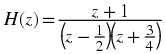
The zeros are: { – 1}
The poles are:
The Z-Plane
Once the poles and zeros have been found for a given Z-Transform, they can be plotted onto the Z-Plane. The Z-plane is a complex plane with an imaginary and real axis referring to the complex-valued variable z . The position on the complex plane is given by r ⅇ ⅈθ and the angle from the positive, real axis around the plane is denoted by θ . When mapping poles and zeros onto the plane, poles are denoted by an "x" and zeros by an "o". The below figure shows the Z-Plane, and examples of plotting zeros and poles onto the plane can be found in the following section.
Figure 12.12. Z-Plane
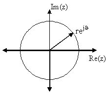
Examples of Pole/Zero Plots
This section lists several examples of finding the poles and zeros of a transfer function and then plotting them onto the Z-Plane.
Example 12.8. Simple Pole/Zero Plot

The zeros are: {0}
The poles are:
Figure 12.13. Pole/Zero Plot
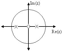
Using the zeros and poles found from the transfer function, the one zero is mapped to zero and the two poles are placed atand

Example 12.9. Complex Pole/Zero Plot
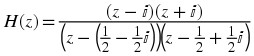
The zeros are: {ⅈ, – ⅈ}
The poles are:
Figure 12.14. Pole/Zero Plot
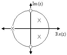
Using the zeros and poles found from the transfer function, the zeros are mapped to ± ⅈ , and the poles are placed at – 1,and

Example 12.10. Pole-Zero Cancellation
An easy mistake to make with regards to poles and zeros is to think that a function likeis the same as s + 3 . In theory they are equivalent, as the pole and zero at s = 1 cancel each other out in what is known as pole-zero cancellation. However, think about what may happen if this were a transfer function of a system that was created with physical circuits. In this case, it is very unlikely that the pole and zero would remain in exactly the same place. A minor temperature change, for instance, could cause one of them to move just slightly. If this were to occur a tremendous amount of volatility is created in that area, since there is a change from infinity at the pole to zero at the zero in a very small range of signals. This is generally a very bad way to try to eliminate a pole. A much better way is to use control theory to move the pole to a better place.
Repeated Poles and Zeros
It is possible to have more than one pole or zero at any given point. For instance, the discrete-time transfer function H(z) = z 2 will have two zeros at the origin and the continuous-time functionwill have 25 poles at the origin.
MATLAB - If access to MATLAB is readily available, then you can use its functions to easily create pole/zero plots. Below is a short program that plots the poles and zeros from the above example onto the Z-Plane.
% Set up vector for zeros
z = [j ; -j];
% Set up vector for poles
p = [-1 ; .5+.5j ; .5-.5j];
figure(1);
zplane(z,p);
title('Pole/Zero Plot for Complex Pole/Zero Plot Example');
Interactive Demonstration of Poles and Zeros
Figure 12.15.

Interact (when online) with a Mathematica CDF demonstrating Pole/Zero Plots. To Download, right-click and save target as .cdf.
Applications for pole-zero plots
Stability and Control theory
Now that we have found and plotted the poles and zeros, we must ask what it is that this plot gives us. Basically what we can gather from this is that the magnitude of the transfer function will be larger when it is closer to the poles and smaller when it is closer to the zeros. This provides us with a qualitative understanding of what the system does at various frequencies and is crucial to the discussion of stability.
Pole/Zero Plots and the Region of Convergence
The region of convergence (ROC) for X(z) in the complex Z-plane can be determined from the pole/zero plot. Although several regions of convergence may be possible, where each one corresponds to a different impulse response, there are some choices that are more practical. A ROC can be chosen to make the transfer function causal and/or stable depending on the pole/zero plot.
Filter Properties from ROC
If the ROC extends outward from the outermost pole, then the system is causal.
If the ROC includes the unit circle, then the system is stable.
Below is a pole/zero plot with a possible ROC of the Z-transform in the Simple Pole/Zero Plot discussed earlier. The shaded region indicates the ROC chosen for the filter. From this figure, we can see that the filter will be both causal and stable since the above listed conditions are both met.
Example 12.11.
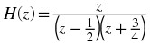
Figure 12.16. Region of Convergence for the Pole/Zero Plot
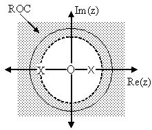
The shaded area represents the chosen ROC for the transfer function.
Frequency Response and Pole/Zero Plots
The reason it is helpful to understand and create these pole/zero plots is due to their ability to help us easily design a filter. Based on the location of the poles and zeros, the magnitude response of the filter can be quickly understood. Also, by starting with the pole/zero plot, one can design a filter and obtain its transfer function very easily.
12.6. Region of Convergence for the Z-transform*
Introduction
With the z-transform, the s-plane represents a set of signals (complex exponentials). For any given LTI system, some of these signals may cause the output of the system to converge, while others cause the output to diverge ("blow up"). The set of signals that cause the system's output to converge lie in the region of convergence (ROC). This module will discuss how to find this region of convergence for any discrete-time, LTI system.
The Region of Convergence
The region of convergence, known as the ROC, is important to understand because it defines the region where the z-transform exists. The z-transform of a sequence is defined as  The ROC for a given x[n] , is defined as the range of z for which the z-transform converges. Since the z-transform is a power series, it converges when x[n]z
– n
is absolutely summable. Stated differently,
The ROC for a given x[n] , is defined as the range of z for which the z-transform converges. Since the z-transform is a power series, it converges when x[n]z
– n
is absolutely summable. Stated differently,  must be satisfied for convergence.
Properties of the Region of Convergencec
The Region of Convergence has a number of properties that are dependent on the characteristics of the signal, x[n] .
The ROC cannot contain any poles. By definition a pole is a where X(z) is infinite. Since X(z) must be finite for all z for convergence, there cannot be a pole in the ROC.
If x[n] is a finite-duration sequence, then the ROC is the entire z-plane, except possibly z = 0 or |z| = ∞ . A finite-duration sequence is a sequence that is nonzero in a finite interval n1 ≤ n ≤ n2 . As long as each value of x[n] is finite then the sequence will be absolutely summable. When n 2 > 0 there will be a z -1 term and thus the ROC will not include z = 0 . When n 1 < 0 then the sum will be infinite and thus the ROC will not include |z| = ∞ . On the other hand, when n 2 ≤ 0 then the ROC will include z = 0 , and when n 1 ≥ 0 the ROC will include |z| = ∞ . With these constraints, the only signal, then, whose ROC is the entire z-plane is x[n] = c δ[n] .
Figure 12.17.

An example of a finite duration sequence.
The next properties apply to infinite duration sequences. As noted above, the z-transform converges when |X(z)| < ∞ . So we can write  We can then split the infinite sum into positive-time and negative-time portions. So |X(z)| ≤ N(z) + P(z) where
 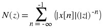 and
and 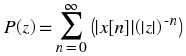 In order for |X(z)| to be finite, |x[n]| must be bounded. Let us then set |x(n)| ≤ C
1
r
1
n
for n < 0 and |x(n)| ≤ C
2
r
2
n
for n ≥ 0 From this some further properties can be derived:
In order for |X(z)| to be finite, |x[n]| must be bounded. Let us then set |x(n)| ≤ C
1
r
1
n
for n < 0 and |x(n)| ≤ C
2
r
2
n
for n ≥ 0 From this some further properties can be derived:
If x[n] is a right-sided sequence, then the ROC extends outward from the outermost pole in X(z) . A right-sided sequence is a sequence where x[n] = 0 for n < n1 < ∞ . Looking at the positive-time portion from the above derivation, it follows that
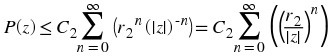 Thus in order for this sum to converge, |z| > r
2 , and therefore the ROC of a right-sided sequence is of the form |z| > r
2 .
Thus in order for this sum to converge, |z| > r
2 , and therefore the ROC of a right-sided sequence is of the form |z| > r
2 .
Figure 12.18.
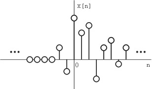
A right-sided sequence.
Figure 12.19.
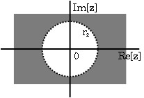
The ROC of a right-sided sequence.
If x[n] is a left-sided sequence, then the ROC extends inward from the innermost pole in X(z) . A left-sided sequence is a sequence where x[n] = 0 for n > n2 > – ∞ . Looking at the negative-time portion from the above derivation, it follows that
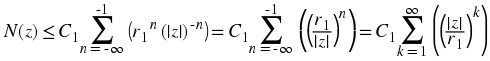 Thus in order for this sum to converge, |z| < r
1 , and therefore the ROC of a left-sided sequence is of the form |z| < r
1 .
Thus in order for this sum to converge, |z| < r
1 , and therefore the ROC of a left-sided sequence is of the form |z| < r
1 .
Figure 12.20.
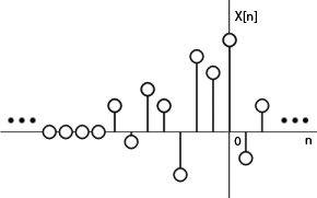
A left-sided sequence.
Figure 12.21.
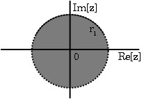
The ROC of a left-sided sequence.
If x[n] is a two-sided sequence, the ROC will be a ring in the z-plane that is bounded on the interior and exterior by a pole. A two-sided sequence is an sequence with infinite duration in the positive and negative directions. From the derivation of the above two properties, it follows that if -r2 < |z| < r 2 converges, then both the positive-time and negative-time portions converge and thus X(z) converges as well. Therefore the ROC of a two-sided sequence is of the form -r2 < |z| < r 2 .
Figure 12.22.
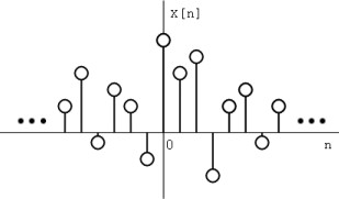
A two-sided sequence.
Figure 12.23.
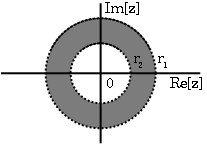
The ROC of a two-sided sequence.
Examples
Example 12.12.
Lets takeThe z-transform of
is
with an ROC at
.
Figure 12.24.
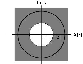
The ROC of

The z-transform ofis
with an ROC at
.
Figure 12.25.
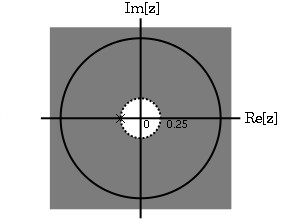
The ROC of

Due to linearity,By observation it is clear that there are two zeros, at 0 and
, and two poles, at
, and
. Following the obove properties, the ROC is
.
Figure 12.26.
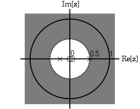
The ROC of
Example 12.13.
Now takeThe z-transform and ROC of
was shown in the example above. The z-transorm of
is
with an ROC at
.
Figure 12.27.

The ROC of
Once again, by linearity,By observation it is again clear that there are two zeros, at 0 and
, and two poles, at
, and
. in ths case though, the ROC is
.
Figure 12.28.
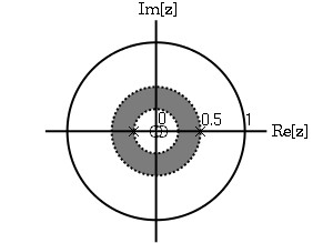
The ROC of.
Graphical Understanding of ROC
Using the demonstration, learn about the region of convergence for the Laplace Transform.
Conclusion
Clearly, in order to craft a system that is actually useful by virtue of being causal and BIBO stable, we must ensure that it is within the Region of Convergence, which can be ascertained by looking at the pole zero plot. The Region of Convergence is the area in the pole/zero plot of the transfer function in which the function exists. For purposes of useful filter design, we prefer to work with rational functions, which can be described by two polynomials, one each for determining the poles and the zeros, respectively.
12.7. Rational Functions and the Z-Transform*
Introduction
When dealing with operations on polynomials, the term rational function is a simple way to describe a particular relationship between two polynomials.
Definition: rational function
For any two polynomials, A and B, their quotient is called a rational function.
Example .
Below is a simple example of a basic rational function, f(x) . Note that the numerator and denominator can be polynomials of any order, but the rational function is undefined when the denominator equals zero.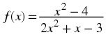
If you have begun to study the Z-transform, you should have noticed by now they are all rational functions. Below we will look at some of the properties of rational functions and how they can be used to reveal important characteristics about a z-transform, and thus a signal or LTI system.
Properties of Rational Functions
In order to see what makes rational functions special, let us look at some of their basic properties and characteristics. If you are familiar with rational functions and basic algebraic properties, skip to the next section to see how rational functions are useful when dealing with the z-transform.
Roots
To understand many of the following characteristics of a rational function, one must begin by finding the roots of the rational function. In order to do this, let us factor both of the polynomials so that the roots can be easily determined. Like all polynomials, the roots will provide us with information on many key properties. The function below shows the results of factoring the above rational function, Equation.
(12.17)
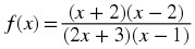
Thus, the roots of the rational function are as follows:
Roots of the numerator are: {-2, 2}
Roots of the denominator are: {-3, 1}
Note
In order to understand rational functions, it is essential to know and understand the roots that make up the rational function.
Discontinuities
Because we are dealing with division of two polynomials, we must be aware of the values of the variable that will cause the denominator of our fraction to be zero. When this happens, the rational function becomes undefined, i.e. we have a discontinuity in the function. Because we have already solved for our roots, it is very easy to see when this occurs. When the variable in the denominator equals any of the roots of the denominator, the function becomes undefined.
Example 12.15.
Continuing to look at our rational function above, Equation, we can see that the function will have discontinuities at the following points:
In respect to the Cartesian plane, we say that the discontinuities are the values along the x-axis where the function is undefined. These discontinuities often appear as vertical asymptotes on the graph to represent the values where the function is undefined.
Domain
Using the roots that we found above, the domain of the rational function can be easily defined.
Definition: domain
The group, or set, of values that are defined by a given function.
Example .
Using the rational function above, Equation, the domain can be defined as any real number x where x does not equal 1 or negative 3. Written out mathematical, we get the following:

Intercepts
The x-intercept is defined as the point(s) where f(x) , i.e. the output of the rational functions, equals zero. Because we have already found the roots of the equation this process is very simple. From algebra, we know that the output will be zero whenever the numerator of the rational function is equal to zero. Therefore, the function will have an x-intercept wherever x equals one of the roots of the numerator.
The y-intercept occurs whenever x equals zero. This can be found by setting all the values of x equal to zero and solving the rational function.
Rational Functions and the Z-Transform
As we have stated above, all z-transforms can be written as rational functions, which have become the most common way of representing the z-transform. Because of this, we can use the properties above, especially those of the roots, in order to reveal certain characteristics about the signal or LTI system described by the z-transform.
Below is the general form of the z-transform written as a rational function: 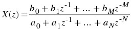 If you have already looked at the module about Understanding Pole/Zero Plots and the Z-transform, you should see how the roots of the rational function play an important role in understanding the z-transform. The equation above, Equation, can be expressed in factored form just as was done for the simple rational function above, see Equation 12.17. Thus, we can easily find the roots of the numerator and denominator of the z-transform. The following two relationships become apparent:
Relationship of Roots to Poles and Zeros
The roots of the numerator in the rational function will be the zeros of the z-transform
The roots of the denominator in the rational function will be the poles of the z-transform
Conclusion
Once we have used our knowledge of rational functions to find its roots, we can manipulate a z-transform in a number of useful ways. We can apply this knowledge to representing an LTI system graphically through a Pole/Zero Plot, or to analyze and design a digital filter through Filter Design from the Z-Transform.
12.8. Difference Equations*
Introduction
One of the most important concepts of DSP is to be able to properly represent the input/output relationship to a given LTI system. A linear constant-coefficient difference equation (LCCDE) serves as a way to express just this relationship in a discrete-time system. Writing the sequence of inputs and outputs, which represent the characteristics of the LTI system, as a difference equation help in understanding and manipulating a system.
Definition: difference equation
An equation that shows the relationship between consecutive values of a sequence and the differences among them. They are often rearranged as a recursive formula so that a systems output can be computed from the input signal and past outputs.
Example .
y[n] + 7y[n − 1] + 2y[n − 2] = x[n] − 4x[n − 1]
General Formulas for the Difference Equation
As stated briefly in the definition above, a difference equation is a very useful tool in describing and calculating the output of the system described by the formula for a given sample n . The key property of the difference equation is its ability to help easily find the transform, H(z) , of a system. In the following two subsections, we will look at the general form of the difference equation and the general conversion to a z-transform directly from the difference equation.
Difference Equation
The general form of a linear, constant-coefficient difference equation (LCCDE), is shown below: 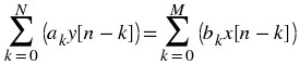 We can also write the general form to easily express a recursive output, which looks like this:
 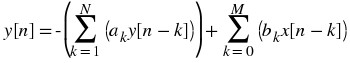 From this equation, note that y[n − k] represents the outputs and x[n − k] represents the inputs. The value of N represents the order of the difference equation and corresponds to the memory of the system being represented. Because this equation relies on past values of the output, in order to compute a numerical solution, certain past outputs, referred to as the initial conditions, must be known.
Conversion to Z-Transform
Using the above formula, Equation, we can easily generalize the transfer function, H(z) , for any difference equation. Below are the steps taken to convert any difference equation into its transfer function, i.e. z-transform. The first step involves taking the Fourier Transform of all the terms in Equation. Then we use the linearity property to pull the transform inside the summation and the time-shifting property of the z-transform to change the time-shifting terms to exponentials. Once this is done, we arrive at the following equation: a
0 = 1 . 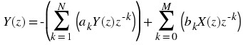
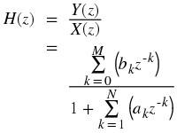
Conversion to Frequency Response
Once the z-transform has been calculated from the difference equation, we can go one step further to define the frequency response of the system, or filter, that is being represented by the difference equation.
Note
Remember that the reason we are dealing with these formulas is to be able to aid us in filter design. A LCCDE is one of the easiest ways to represent FIR filters. By being able to find the frequency response, we will be able to look at the basic properties of any filter represented by a simple LCCDE.
Below is the general formula for the frequency response of a z-transform. The conversion is simple a matter of taking the z-transform formula, H(z) , and replacing every instance of z with ⅇ
ⅈw
. 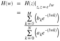 Once you understand the derivation of this formula, look at the module concerning Filter Design from the Z-Transform for a look into how all of these ideas of the Z-transform, Difference Equation, and Pole/Zero Plots play a role in filter design.
Example
Example 12.18. Finding Difference Equation
Below is a basic example showing the opposite of the steps above: given a transfer function one can easily calculate the systems difference equation.Given this transfer function of a time-domain filter, we want to find the difference equation. To begin with, expand both polynomials and divide them by the highest order z .
From this transfer function, the coefficients of the two polynomials will be our a k and b k values found in the general difference equation formula, Equation. Using these coefficients and the above form of the transfer function, we can easily write the difference equation:
In our final step, we can rewrite the difference equation in its more common form showing the recursive nature of the system.

Solving a LCCDE
In order for a linear constant-coefficient difference equation to be useful in analyzing a LTI system, we must be able to find the systems output based upon a known input, x(n) , and a set of initial conditions. Two common methods exist for solving a LCCDE: the direct method and the indirect method, the later being based on the z-transform. Below we will briefly discuss the formulas for solving a LCCDE using each of these methods.
Direct Method
The final solution to the output based on the direct method is the sum of two parts, expressed in the following equation: y(n) = y h (n) + y p (n) The first part, y h (n) , is referred to as the homogeneous solution and the second part, y h (n) , is referred to as particular solution. The following method is very similar to that used to solve many differential equations, so if you have taken a differential calculus course or used differential equations before then this should seem very familiar.
Homogeneous Solution
We begin by assuming that the input is zero, x(n) = 0 . Now we simply need to solve the homogeneous difference equation: 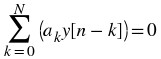 In order to solve this, we will make the assumption that the solution is in the form of an exponential. We will use lambda, λ , to represent our exponential terms. We now have to solve the following equation:
 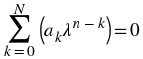 We can expand this equation out and factor out all of the lambda terms. This will give us a large polynomial in parenthesis, which is referred to as the characteristic polynomial. The roots of this polynomial will be the key to solving the homogeneous equation. If there are all distinct roots, then the general solution to the equation will be as follows: y
h
(n) = C
1(λ
1)n
+ C
2(λ
2)n
+ … + C
N
(λ
N
)n
However, if the characteristic equation contains multiple roots then the above general solution will be slightly different. Below we have the modified version for an equation where λ
1
has K multiple roots: y
h
(n) = C
1(λ
1)n
+ C
1
n(λ
1)n
+ C
1
n
2(λ
1)n
+ … + C
1
n
K − 1(λ
1)n
+ C
2(λ
2)n
+ … + C
N
(λ
N
)n
We can expand this equation out and factor out all of the lambda terms. This will give us a large polynomial in parenthesis, which is referred to as the characteristic polynomial. The roots of this polynomial will be the key to solving the homogeneous equation. If there are all distinct roots, then the general solution to the equation will be as follows: y
h
(n) = C
1(λ
1)n
+ C
2(λ
2)n
+ … + C
N
(λ
N
)n
However, if the characteristic equation contains multiple roots then the above general solution will be slightly different. Below we have the modified version for an equation where λ
1
has K multiple roots: y
h
(n) = C
1(λ
1)n
+ C
1
n(λ
1)n
+ C
1
n
2(λ
1)n
+ … + C
1
n
K − 1(λ
1)n
+ C
2(λ
2)n
+ … + C
N
(λ
N
)n
Particular Solution
The particular solution, y
p
(n) , will be any solution that will solve the general difference equation: 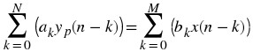 In order to solve, our guess for the solution to y
p
(n) will take on the form of the input, x(n) . After guessing at a solution to the above equation involving the particular solution, one only needs to plug the solution into the difference equation and solve it out.
In order to solve, our guess for the solution to y
p
(n) will take on the form of the input, x(n) . After guessing at a solution to the above equation involving the particular solution, one only needs to plug the solution into the difference equation and solve it out.
Indirect Method
The indirect method utilizes the relationship between the difference equation and z-transform, discussed earlier, to find a solution. The basic idea is to convert the difference equation into a z-transform, as described above, to get the resulting output, Y(z) . Then by inverse transforming this and using partial-fraction expansion, we can arrive at the solution.
(12.18)Z {y ( n + 1 ) – y ( n ) } = z Y ( z ) – y ( 0 )
This can be interatively extended to an arbitrary order derivative as in Equation Equation 12.19.
(12.19)
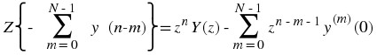
Now, the Laplace transform of each side of the differential equation can be taken
(12.20)
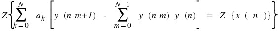
which by linearity results in
(12.21)
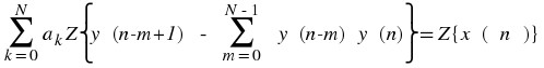
and by differentiation properties in
(12.22)
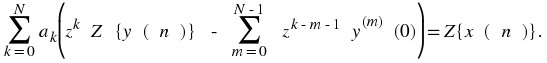
Rearranging terms to isolate the Laplace transform of the output,
(12.23)

Thus, it is found that
(12.24)
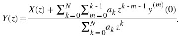
In order to find the output, it only remains to find the Laplace transform X(z) of the input, substitute the initial conditions, and compute the inverse Z-transform of the result. Partial fraction expansions are often required for this last step. This may sound daunting while looking at Equation 12.24, but it is often easy in practice, especially for low order difference equations. Equation 12.24 can also be used to determine the transfer function and frequency response.
As an example, consider the difference equation
(12.25)y [ n - 2 ] + 4 y [ n - 1 ] + 3 y [ n ] = cos ( n )
with the initial conditions y ' (0) = 1 and y(0) = 0 Using the method described above, the Z transform of the solution y[n] is given by
(12.26)
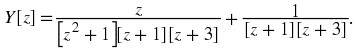
Performing a partial fraction decomposition, this also equals
(12.27)
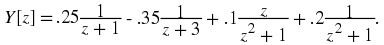
Computing the inverse Laplace transform,
(12.28)

One can check that this satisfies that this satisfies both the differential equation and the initial conditions.
12.9. Discrete Time Filter Design*
Estimating Frequency Response from Z-Plane
One of the primary motivating factors for utilizing the z-transform and analyzing the pole/zero plots is due to their relationship to the frequency response of a discrete-time system. Based on the position of the poles and zeros, one can quickly determine the frequency response. This is a result of the correspondence between the frequency response and the transfer function evaluated on the unit circle in the pole/zero plots. The frequency response, or DTFT, of the system is defined as:  Next, by factoring the transfer function into poles and zeros and multiplying the numerator and denominator by ⅇ
ⅈw
we arrive at the following equations:
Next, by factoring the transfer function into poles and zeros and multiplying the numerator and denominator by ⅇ
ⅈw
we arrive at the following equations:  From Equation we have the frequency response in a form that can be used to interpret physical characteristics about the filter's frequency response. The numerator and denominator contain a product of terms of the form |ⅇ
ⅈw
− h|, where h is either a zero, denoted by c
k
or a pole, denoted by d
k
. Vectors are commonly used to represent the term and its parts on the complex plane. The pole or zero, h , is a vector from the origin to its location anywhere on the complex plane and ⅇ
ⅈw
is a vector from the origin to its location on the unit circle. The vector connecting these two points, |ⅇ
ⅈw
− h|, connects the pole or zero location to a place on the unit circle dependent on the value of w . From this, we can begin to understand how the magnitude of the frequency response is a ratio of the distances to the poles and zero present in the z-plane as w goes from zero to pi. These characteristics allow us to interpret |H(w)| as follows:
From Equation we have the frequency response in a form that can be used to interpret physical characteristics about the filter's frequency response. The numerator and denominator contain a product of terms of the form |ⅇ
ⅈw
− h|, where h is either a zero, denoted by c
k
or a pole, denoted by d
k
. Vectors are commonly used to represent the term and its parts on the complex plane. The pole or zero, h , is a vector from the origin to its location anywhere on the complex plane and ⅇ
ⅈw
is a vector from the origin to its location on the unit circle. The vector connecting these two points, |ⅇ
ⅈw
− h|, connects the pole or zero location to a place on the unit circle dependent on the value of w . From this, we can begin to understand how the magnitude of the frequency response is a ratio of the distances to the poles and zero present in the z-plane as w goes from zero to pi. These characteristics allow us to interpret |H(w)| as follows: 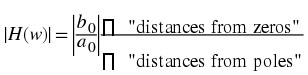
Drawing Frequency Response from Pole/Zero Plot
Let us now look at several examples of determining the magnitude of the frequency response from the pole/zero plot of a z-transform. If you have forgotten or are unfamiliar with pole/zero plots, please refer back to the Pole/Zero Plots module.
Example 12.19.
In this first example we will take a look at the very simple z-transform shown below: H(z) = z + 1 = 1 + z -1 H(w) = 1 + ⅇ – (ⅈw) For this example, some of the vectors represented by |ⅇ ⅈw − h|, for random values of w , are explicitly drawn onto the complex plane shown in the figure below. These vectors show how the amplitude of the frequency response changes as w goes from 0 to 2π , and also show the physical meaning of the terms in Equation above. One can see that when w = 0, the vector is the longest and thus the frequency response will have its largest amplitude here. As w approaches π , the length of the vectors decrease as does the amplitude of |H(w)|. Since there are no poles in the transform, there is only this one vector term rather than a ratio as seen in Equation.
Figure 12.29. Pole/Zero Plot

(a)
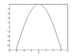
(b)
The first figure represents the pole/zero plot with a few representative vectors graphed while the second shows the frequency response with a peak at +2 and graphed between plus and minus π .
Example 12.20.
For this example, a more complex transfer function is analyzed in order to represent the system's frequency response.
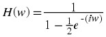
Below we can see the two figures described by the above equations. The Figure 12.30 represents the basic pole/zero plot of the z-transform, H(w). Figure 12.30 shows the magnitude of the frequency response. From the formulas and statements in the previous section, we can see that when w = 0 the frequency will peak since it is at this value of w that the pole is closest to the unit circle. The ratio from Equation helps us see the mathematics behind this conclusion and the relationship between the distances from the unit circle and the poles and zeros. As w moves from 0 to π , we see how the zero begins to mask the effects of the pole and thus force the frequency response closer to 0.
Figure 12.30. Pole/Zero Plot
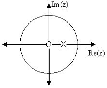
(a)
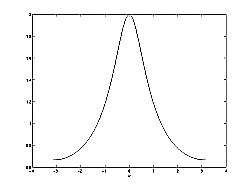
(b)
The first figure represents the pole/zero plot while the second shows the frequency response with a peak at +2 and graphed between plus and minus π .
Interactive Filter Design Illustration
Figure 12.31.
(This media type is not supported in this reader. Click to open media in browser.)
Digital filter design LabVIEW virtual instrument by NI from http://cnx.org/content/m13115/latest/.
Conclusion
In conclusion, using the distances from the unit circle to the poles and zeros, we can plot the frequency response of the system. As w goes from 0 to 2π , the following two properties, taken from the above equations, specify how one should draw |H(w)|.
While moving around the unit circle...
if close to a zero, then the magnitude is small. If a zero is on the unit circle, then the frequency response is zero at that point.
if close to a pole, then the magnitude is large. If a pole is on the unit circle, then the frequency response goes to infinity at that point.
Chapter 13. Capstone Signal Processing Topics
13.1. DFT: Fast Fourier Transform*
We now have a way of computing the spectrum for an arbitrary signal: The Discrete Fourier Transform (DFT) computes the spectrum at N equally spaced frequencies from a length- N sequence. An issue that never arises in analog "computation," like that performed by a circuit, is how much work it takes to perform the signal processing operation such as filtering. In computation, this consideration translates to the number of basic computational steps required to perform the needed processing. The number of steps, known as the complexity, becomes equivalent to how long the computation takes (how long must we wait for an answer). Complexity is not so much tied to specific computers or programming languages but to how many steps are required on any computer. Thus, a procedure's stated complexity says that the time taken will be proportional to some function of the amount of data used in the computation and the amount demanded.
For example, consider the formula for the discrete Fourier transform. For each frequency we chose, we must multiply each signal value by a complex number and add together the results. For a real-valued signal, each real-times-complex multiplication requires two real multiplications, meaning we have 2N multiplications to perform. To add the results together, we must keep the real and imaginary parts separate. Adding N numbers requires N − 1 additions. Consequently, each frequency requires 2N + 2(N − 1) = 4N − 2 basic computational steps. As we have N frequencies, the total number of computations is N(4N − 2) .
In complexity calculations, we only worry about what happens as the data lengths increase, and take the dominant term—here the 4N 2 term—as reflecting how much work is involved in making the computation. As multiplicative constants don't matter since we are making a "proportional to" evaluation, we find the DFT is an O(N 2) computational procedure. This notation is read "order N -squared". Thus, if we double the length of the data, we would expect that the computation time to approximately quadruple.
Exercise 13.1.1. (Go to Solution)
In making the complexity evaluation for the DFT, we assumed the data to be real. Three questions emerge. First of all, the spectra of such signals have conjugate symmetry, meaning that negative frequency components ( in the DFT) can be computed from the corresponding positive frequency components. Does this symmetry change the DFT's complexity?
Secondly, suppose the data are complex-valued; what is the DFT's complexity now?
Finally, a less important but interesting question is suppose we want K frequency values instead of N ; now what is the complexity?
Solutions to Exercises
Solution to Exercise 13.1.1. (Return to Exercise)
When the signal is real-valued, we may only need half the spectral values, but the complexity remains unchanged. If the data are complex-valued, which demands retaining all frequency values, the complexity is again the same. When only K frequencies are needed, the complexity is O(KN) .
13.2. The Fast Fourier Transform (FFT)*
Introduction
The Fast Fourier Transform (FFT) is an efficient O(NlogN) algorithm for calculating DFTs The FFT exploits symmetries in the W matrix to take a "divide and conquer" approach. We will first discuss deriving the actual FFT algorithm, some of its implications for the DFT, and a speed comparison to drive home the importance of this powerful algorithm.
Deriving the FFT
To derive the FFT, we assume that the signal's duration is a power of two: N = 2l . Consider what happens to the even-numbered and odd-numbered elements of the sequence in the DFT calculation.
(13.1)

Each term in square brackets has the form of a  -length DFT. The first one is a DFT of the even-numbered elements, and the second of the odd-numbered elements. The first DFT is combined with the second multiplied by the complex exponential
  . The half-length transforms are each evaluated at frequency indices k ∈ {0, …, N − 1} . Normally, the number of frequency indices in a DFT calculation range between zero and the transform length minus one. The computational advantage of the FFT comes from recognizing the periodic nature of the discrete Fourier transform. The FFT simply reuses the computations made in the half-length transforms and combines them through additions and the multiplication by
  , which is not periodic over
  , to rewrite the length-N DFT. Figure 13.1 illustrates this decomposition. As it stands, we now compute two length-
  transforms (complexity
  ), multiply one of them by the complex exponential (complexity O(N) ), and add the results (complexity O(N) ). At this point, the total complexity is still dominated by the half-length DFT calculations, but the proportionality coefficient has been reduced.
Now for the fun. Because N = 2l
, each of the half-length transforms can be reduced to two quarter-length transforms, each of these to two eighth-length ones, etc. This decomposition continues until we are left with length-2 transforms. This transform is quite simple, involving only additions. Thus, the first stage of the FFT has  length-2 transforms (see the bottom part of Figure 13.1). Pairs of these transforms are combined by adding one to the other multiplied by a complex exponential. Each pair requires 4 additions and 4 multiplications, giving a total number of computations equaling
  . This number of computations does not change from stage to stage. Because the number of stages, the number of times the length can be divided by two, equals log2
N , the complexity of the FFT is O(N
logN) .
. This number of computations does not change from stage to stage. Because the number of stages, the number of times the length can be divided by two, equals log2
N , the complexity of the FFT is O(N
logN) .
Figure 13.1. Length-8 DFT decomposition
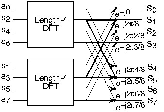
(a)

(b)
The initial decomposition of a length-8 DFT into the terms using even- and odd-indexed inputs marks the first phase of developing the FFT algorithm. When these half-length transforms are successively decomposed, we are left with the diagram shown in the bottom panel that depicts the length-8 FFT computation.
Doing an example will make computational savings more obvious. Let's look at the details of a length-8 DFT. As shown on Figure 13.1, we first decompose the DFT into two length-4 DFTs, with the outputs added and subtracted together in pairs. Considering Figure 13.1 as the frequency index goes from 0 through 7, we recycle values from the length-4 DFTs into the final calculation because of the periodicity of the DFT output. Examining how pairs of outputs are collected together, we create the basic computational element known as a butterfly (Figure 13.2).
Figure 13.2. Butterfly

The basic computational element of the fast Fourier transform is the butterfly. It takes two complex numbers, represented by a and b, and forms the quantities shown. Each butterfly requires one complex multiplication and two complex additions.
By considering together the computations involving common output frequencies from the two half-length DFTs, we see that the two complex multiplies are related to each other, and we can reduce our computational work even further. By further decomposing the length-4 DFTs into two length-2 DFTs and combining their outputs, we arrive at the diagram summarizing the length-8 fast Fourier transform (Figure 13.1). Although most of the complex multiplies are quite simple (multiplying by ⅇ
– (ⅈπ) means negating real and imaginary parts), let's count those for purposes of evaluating the complexity as full complex multiplies. We have  complex multiplies and 2N = 16 additions for each stage and log2
N = 3 stages, making the number of basic computations
complex multiplies and 2N = 16 additions for each stage and log2
N = 3 stages, making the number of basic computations  as predicted.
Exercise 13.2.1. (Go to Solution)
Note that the ordering of the input sequence in the two parts of Figure 13.1 aren't quite the same. Why not? How is the ordering determined?
FFT and the DFT
We now have a way of computing the spectrum for an arbitrary signal: The Discrete Fourier Transform (DFT) computes the spectrum at N equally spaced frequencies from a length- N sequence. An issue that never arises in analog "computation," like that performed by a circuit, is how much work it takes to perform the signal processing operation such as filtering. In computation, this consideration translates to the number of basic computational steps required to perform the needed processing. The number of steps, known as the complexity, becomes equivalent to how long the computation takes (how long must we wait for an answer). Complexity is not so much tied to specific computers or programming languages but to how many steps are required on any computer. Thus, a procedure's stated complexity says that the time taken will be proportional to some function of the amount of data used in the computation and the amount demanded.
For example, consider the formula for the discrete Fourier transform. For each frequency we chose, we must multiply each signal value by a complex number and add together the results. For a real-valued signal, each real-times-complex multiplication requires two real multiplications, meaning we have 2N multiplications to perform. To add the results together, we must keep the real and imaginary parts separate. Adding N numbers requires N − 1 additions. Consequently, each frequency requires 2N + 2(N − 1) = 4N − 2 basic computational steps. As we have N frequencies, the total number of computations is N(4N − 2) .
In complexity calculations, we only worry about what happens as the data lengths increase, and take the dominant term—here the 4N 2 term—as reflecting how much work is involved in making the computation. As multiplicative constants don't matter since we are making a "proportional to" evaluation, we find the DFT is an O(N 2) computational procedure. This notation is read "order N -squared". Thus, if we double the length of the data, we would expect that the computation time to approximately quadruple.
Exercise 13.2.2. (Go to Solution)
In making the complexity evaluation for the DFT, we assumed the data to be real. Three questions emerge. First of all, the spectra of such signals have conjugate symmetry, meaning that negative frequency components ( in the DFT) can be computed from the corresponding positive frequency components. Does this symmetry change the DFT's complexity?
Secondly, suppose the data are complex-valued; what is the DFT's complexity now?
Finally, a less important but interesting question is suppose we want K frequency values instead of N ; now what is the complexity?
Speed Comparison
How much better is O(NlogN) than O( N 2 )?
Figure 13.3.
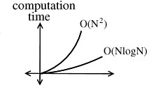
This figure shows how much slower the computation time of an O(NlogN) process grows.
| N | 10 | 100 | 1000 | 10 6 | 10 9 |
|---|---|---|---|---|---|
| N 2 | 100 | 10 4 | 10 6 | 10 12 | 10 18 |
| N logN | 1 | 200 | 3000 | 6 × 10 6 | 9 × 10 9 |
Say you have a 1 MFLOP machine (a million "floating point" operations per second). Let N = 1million = 106 .
An O( N 2 ) algorithm takes 1012 flors → 106 seconds ≃ 11.5 days.
An O( N logN ) algorithm takes 6 × 10⁶ Flors → 6 seconds.
Note
N = 1million is not unreasonable.
Example 13.1.
3 megapixel digital camera spits out 3 × 10⁶ numbers for each picture. So for two N point sequences f[n] and h[n]. If computing (f[n] ⊛ h[n]) directly: O( N 2 ) operations.
taking FFTs -- O(NlogN)
multiplying FFTs -- O(N)
inverse FFTs -- O(NlogN).
the total complexity is O(NlogN).
Conclusion
Other "fast" algorithms have been discovered, most of which make use of how many common factors the transform length N has. In number theory, the number of prime factors a given integer has measures how composite it is. The numbers 16 and 81 are highly composite (equaling 24 and 34 respectively), the number 18 is less so ( 2132 ), and 17 not at all (it's prime). In over thirty years of Fourier transform algorithm development, the original Cooley-Tukey algorithm is far and away the most frequently used. It is so computationally efficient that power-of-two transform lengths are frequently used regardless of what the actual length of the data. It is even well established that the FFT, alongside the digital computer, were almost completely responsible for the "explosion" of DSP in the 60's.
Solutions to Exercises
Solution to Exercise 13.2.1. (Return to Exercise)
The upper panel has not used the FFT algorithm to compute the length-4 DFTs while the lower one has. The ordering is determined by the algorithm.
Solution to Exercise 13.2.2. (Return to Exercise)
When the signal is real-valued, we may only need half the spectral values, but the complexity remains unchanged. If the data are complex-valued, which demands retaining all frequency values, the complexity is again the same. When only K frequencies are needed, the complexity is O(KN) .
13.3. Deriving the Fast Fourier Transform*
To derive the FFT, we assume that the signal's duration is a power of two: N = 2l . Consider what happens to the even-numbered and odd-numbered elements of the sequence in the DFT calculation.
(13.2)
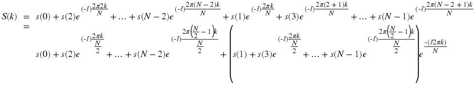
Each term in square brackets has the form of a  -length DFT. The first one is a DFT of the even-numbered elements, and the second of the odd-numbered elements. The first DFT is combined with the second multiplied by the complex exponential
  . The half-length transforms are each evaluated at frequency indices k ∈ {0, …, N − 1} . Normally, the number of frequency indices in a DFT calculation range between zero and the transform length minus one. The computational advantage of the FFT comes from recognizing the periodic nature of the discrete Fourier transform. The FFT simply reuses the computations made in the half-length transforms and combines them through additions and the multiplication by
  , which is not periodic over
  , to rewrite the length-N DFT. Figure 13.4 illustrates this decomposition. As it stands, we now compute two length-
  transforms (complexity
  ), multiply one of them by the complex exponential (complexity O(N) ), and add the results (complexity O(N) ). At this point, the total complexity is still dominated by the half-length DFT calculations, but the proportionality coefficient has been reduced.
Now for the fun. Because N = 2l
, each of the half-length transforms can be reduced to two quarter-length transforms, each of these to two eighth-length ones, etc. This decomposition continues until we are left with length-2 transforms. This transform is quite simple, involving only additions. Thus, the first stage of the FFT has  length-2 transforms (see the bottom part of Figure 13.4). Pairs of these transforms are combined by adding one to the other multiplied by a complex exponential. Each pair requires 4 additions and 4 multiplications, giving a total number of computations equaling
  . This number of computations does not change from stage to stage. Because the number of stages, the number of times the length can be divided by two, equals log2
N , the complexity of the FFT is O(N
logN) .
. This number of computations does not change from stage to stage. Because the number of stages, the number of times the length can be divided by two, equals log2
N , the complexity of the FFT is O(N
logN) .
Figure 13.4. Length-8 DFT decomposition

(a)
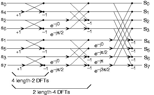
(b)
The initial decomposition of a length-8 DFT into the terms using even- and odd-indexed inputs marks the first phase of developing the FFT algorithm. When these half-length transforms are successively decomposed, we are left with the diagram shown in the bottom panel that depicts the length-8 FFT computation.
Doing an example will make computational savings more obvious. Let's look at the details of a length-8 DFT. As shown on Figure 13.4, we first decompose the DFT into two length-4 DFTs, with the outputs added and subtracted together in pairs. Considering Figure 13.4 as the frequency index goes from 0 through 7, we recycle values from the length-4 DFTs into the final calculation because of the periodicity of the DFT output. Examining how pairs of outputs are collected together, we create the basic computational element known as a butterfly (Figure 13.5).
Figure 13.5. Butterfly

The basic computational element of the fast Fourier transform is the butterfly. It takes two complex numbers, represented by a and b, and forms the quantities shown. Each butterfly requires one complex multiplication and two complex additions.
By considering together the computations involving common output frequencies from the two half-length DFTs, we see that the two complex multiplies are related to each other, and we can reduce our computational work even further. By further decomposing the length-4 DFTs into two length-2 DFTs and combining their outputs, we arrive at the diagram summarizing the length-8 fast Fourier transform (Figure 13.4). Although most of the complex multiplies are quite simple (multiplying by ⅇ
– (ⅈπ) means negating real and imaginary parts), let's count those for purposes of evaluating the complexity as full complex multiplies. We have  complex multiplies and 2N = 16 additions for each stage and log2
N = 3 stages, making the number of basic computations
complex multiplies and 2N = 16 additions for each stage and log2
N = 3 stages, making the number of basic computations  as predicted.
Exercise 13.3.1. (Go to Solution)
Note that the ordering of the input sequence in the two parts of Figure 13.4 aren't quite the same. Why not? How is the ordering determined?
Other "fast" algorithms were discovered, all of which make use of how many common factors the transform length N has. In number theory, the number of prime factors a given integer has measures how composite it is. The numbers 16 and 81 are highly composite (equaling 24 and 34 respectively), the number 18 is less so ( 2132 ), and 17 not at all (it's prime). In over thirty years of Fourier transform algorithm development, the original Cooley-Tukey algorithm is far and away the most frequently used. It is so computationally efficient that power-of-two transform lengths are frequently used regardless of what the actual length of the data.
Solutions to Exercises
Solution to Exercise 13.3.1. (Return to Exercise)
The upper panel has not used the FFT algorithm to compute the length-4 DFTs while the lower one has. The ordering is determined by the algorithm.
13.4. Matched Filter Detector*
Introduction
A great many applications in signal processing, image processing, and beyond involve determining the presence and location of a target signal within some other signal. A radar system, for example, searches for copies of a transmitted radar pulse in order to determine the presence of and distance to reflective objects such as buildings or aircraft. A communication system searches for copies of waveforms representing digital 0s and 1s in order to receive a message.
Two key mathematical tools that contribute to these applications are inner products and the Cauchy-Schwarz inequality. As is shown in the module on the Cauchy-Schwarz inequality, the expression  attains its upper bound, which is 1, when y = a
x for some scalar a in a real or complex field. The lower bound, which is 0, is attained when x and y are orthogonal. In informal intuition, this means that the expression is maximized when the vectors x and y have the same shape or pattern and minimized when x and y are very different. A pair of vectors with similar but unequal shapes or patterns will produce relatively large value of the expression less than 1, and a pair of vectors with very different but not orthogonal shapes or patterns will produce relatively small values of the expression greater than 0. Thus, the above expression carries with it a notion of the degree to which two signals are “alike”, the magnitude of the normalized correlation between the signals in the case of the standard inner products.
attains its upper bound, which is 1, when y = a
x for some scalar a in a real or complex field. The lower bound, which is 0, is attained when x and y are orthogonal. In informal intuition, this means that the expression is maximized when the vectors x and y have the same shape or pattern and minimized when x and y are very different. A pair of vectors with similar but unequal shapes or patterns will produce relatively large value of the expression less than 1, and a pair of vectors with very different but not orthogonal shapes or patterns will produce relatively small values of the expression greater than 0. Thus, the above expression carries with it a notion of the degree to which two signals are “alike”, the magnitude of the normalized correlation between the signals in the case of the standard inner products.
This concept can be extremely useful. For instance consider a situation in which we wish to determine which signal, if any, from a set X of signals most resembles a particular signal y . In order to accomplish this, we might evaluate the above expression for every signal x ∈ X , choosing the one that results in maxima provided that those maxima are above some threshold of “likeness”. This is the idea behind the matched filter detector, which compares a set of signals against a target signal using the above expression in order to determine which is most like the target signal.
Matched Filter Detector Theory
Signal Comparison
The simplest variant of the matched filter detector scheme would be to find the member signal in a set X of signals that most closely matches a target signal y . Thus, for every x ∈ X we wish to evaluate
(13.3)
in order to compare every member of X to the target signal y . Since the member of X which most closely matches the target signal y is desired, ultimately we wish to evaluate
(13.4)
Note that the target signal does not technically need to be normalized to produce a maximum, but gives the desirable property that m(x,y) is bounded to [0,1].
The element x m ∈ X that produces the maximum value of m(x,y) is not necessarily unique, so there may be more than one matching signal in X . Additionally, the signal x m ∈ X producing the maximum value of m(x,y) may not produce a very large value of m(x,y) and thus not be very much like the target signal y . Hence, another matched filter scheme might identify the argument producing the maximum but only above a certain threshold, returning no matching signals in X if the maximum is below the threshold. There also may be a signal x ∈ X that produces a large value of m(x,y) and thus has a high degree of “likeness” to y but does not produce the maximum value of m(x,y). Thus, yet another matched filter scheme might identify all signals in X producing local maxima that are above a certain threshold.
Example 13.2.
For example, consider the target signal given in Figure 13.6 and the set of two signals given in Figure 13.7. By inspection, it is clear that the signal g 2 is most like the target signal f . However, to make that conclusion mathematically, we use the matched filter detector with the L 2 inner product. If we were to actually make the necessary computations, we would first normalize each signal and then compute the necessary inner products in order to compare the signals in X with the target signal f . We would notice that the absolute value of the inner product for g 2 with f when normalized is greater than the absolute value of the inner product of g 1 with f when normalized, mathematically stated as
(13.5)
Figure 13.6. Template Signal

We wish to find a match for this target signal in the set of signals below.
Figure 13.7. Candidate Signals

(a)
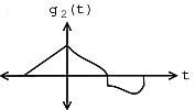
(b)
We wish to find a match for the above target signal in this set of signals.
Pattern Detection
A somewhat more involved matched filter detector scheme would involve attempting to match a target time limited signal y = f to a set of of time shifted and windowed versions of a single signal 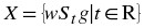 indexed by R. The windowing funtion is given by
  where
where  is the interval to which f is time limited. This scheme could be used to find portions of g that have the same shape as f . If the absolute value of the inner product of the normalized versions of f and w
S
t
g is large, which is the absolute value of the normalized correlation for standard inner products, then g has a high degree of “likeness” to f on the interval to which f is time limited but left shifted by t . Of course, if f is not time limited, it means that the entire signal has a high degree of “likeness” to f left shifted by t .
is the interval to which f is time limited. This scheme could be used to find portions of g that have the same shape as f . If the absolute value of the inner product of the normalized versions of f and w
S
t
g is large, which is the absolute value of the normalized correlation for standard inner products, then g has a high degree of “likeness” to f on the interval to which f is time limited but left shifted by t . Of course, if f is not time limited, it means that the entire signal has a high degree of “likeness” to f left shifted by t .
Thus, in order to determine the most likely locations of a signal with the same shape as the target signal f in a signal g we wish to compute
(13.6)
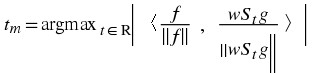
to provide the desired shift. Assuming the inner product space examined is L 2(R (similar results hold for L 2(R[a,b)), l 2(Z), and l 2(Z[a,b))), this produces
(13.7)
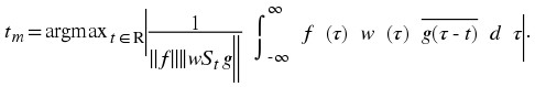
Since f and w are time limited to the same interval
(13.8)

Making the subsitution  ,
,
(13.9)
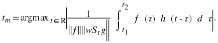
Noting that this expression contains a convolution operation
(13.10)
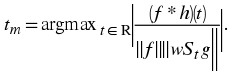
where h is the conjugate of the time reversed version of g defined by 
In the special case in which the target signal f is not time limited, w has unit value on the entire real line. Thus, the norm can be evaluated as ||w
S
t
g|| = ||S
t
g|| = ||g|| = ||h||. Therefore, the function reduces to 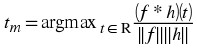 where
where 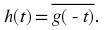 The function
 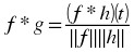 is known as the normalized cross-correlation of f and g .
Hence, this matched filter scheme can be implemented as a convolution. Therefore, it may be expedient to implement it in the frequency domain. Similar results hold for the L 2(R[a,b)), l 2(Z), and l 2(Z[a,b]) spaces. It is especially useful to implement the l 2(Z[a,b]) cases in the frequency domain as the power of the Fast Fourier Transform algorithm can be leveraged to quickly perform the computations in a computer program. In the L 2(R[a,b)) and l 2(Z[a,b]) cases, care must be taken to zero pad the signal if wrap-around effects are not desired. Similar results also hold for spaces on higher dimensional intervals with the same inner products.
Of course, there is not necessarily exactly one instance of a target signal in a given signal. There could be one instance, more than one instance, or no instance of a target signal. Therefore, it is often more practical to identify all shifts corresponding to local maxima that are above a certain threshold.
Example 13.3.
The signal in Figure 13.9 contains an instance of the template signal seen in Figure 13.8 beginning at time t = s 1 as shown by the plot in Figure 13.10. Therefore,
(13.11)
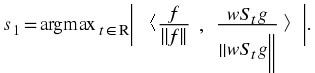
Figure 13.8. Pattern Signal

This function shows tha pattern we are looking for in the signal below, which occurs at time t = s 1 .
Figure 13.9. Longer Signal
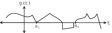
This signal contains an instance of the above signal starting at time t = s 1 .
Figure 13.10. Absolute Value of Output

This signal shows a sketch of the absolute value of the matched filter output for the interval shown. Note that this was just an "eyeball approximation" sketch. Observe the pronounced peak at time t = s 1 .
Practical Applications
Image Detection
Matched Filtering is used in image processing to detect a template image within a reference image. This has real-word applications in verifying fingerprints for security or in verifying someone's photo. As a simple example, we can turn to the ever-popular "Where's Waldo?" books (known as Wally in the UK!), where the reader is tasked with finding the specific face of Waldo/Wally in a confusing background rife with look-alikes! If we are given the template head and a reference image, we can run a two dimensional convolution of the template image across the reference image to obtain a three dimensional convolution map, Figure 13.11, where the height of the convolution map is determined by the degree of correlation, higher being more correlated. Finding our target then becomes a matter of determining the spot where the local surface area is highest. The process is demonstrated in Figure 13.11. In the field of image processing, this matched filter-based process is known as template matching.
Figure 13.11.
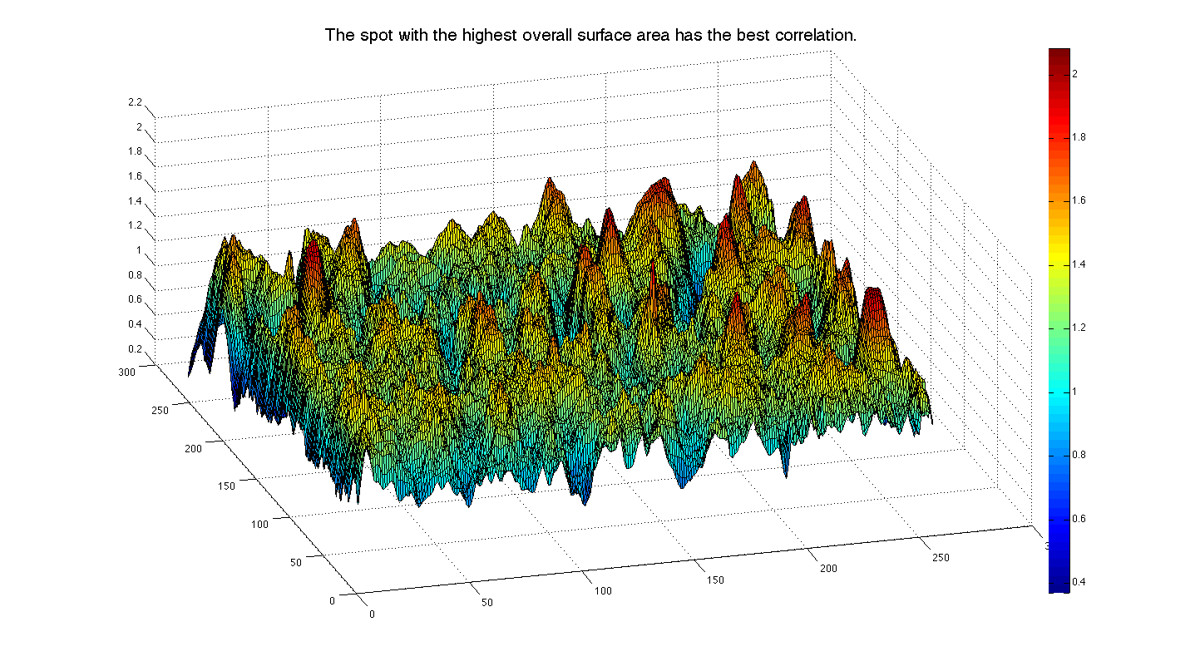
(a)
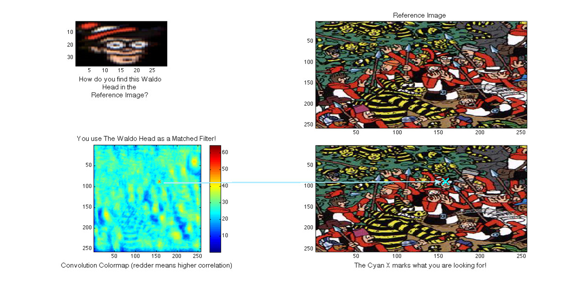
(b)
Example of "Where's Waldo?" picture. Our Matched Filter Detector can be implemented to find a possible match for Waldo.
then we could easily develop a program to find the closest resemblance to the image of Waldo's head in the larger picture. We would simply implement our same match filter algorithm: take the inner products at each shift and see how large our resulting answers are. This idea was implemented on this same picture for a Signals and Systems Project at Rice University (click the link to learn more).
Exercise 13.4.1. Pros and Cons (Go to Solution)
What are the advantages of the matched filter algorithm to image detection? What are the drawbacks of this method?
Communications Systems
Matched filter detectors are also commonly used in Communications Systems. In fact, they are the optimal detectors in Gaussian noise. Signals in the real-world are often distorted by the environment around them, so there is a constant struggle to develop ways to be able to receive a distorted signal and then be able to filter it in some way to determine what the original signal was. Matched filters provide one way to compare a received signal with two possible original ("template") signals and determine which one is the closest match to the received signal.
For example, below we have a simplified example of Frequency Shift Keying (FSK) where we having the following coding for '1' and '0':
Figure 13.12.
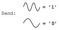
Frequency Shift Keying for '1' and '0'.
Based on the above coding, we can create digital signals based on 0's and 1's by putting together the above two "codes" in an infinite number of ways. For this example we will transmit a basic 3-bit number, 101, which is displayed in Figure 13.13:
Figure 13.13.
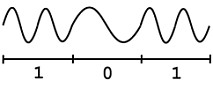
The bit stream "101" coded with the above FSK.
Now, the signal picture above represents our original signal that will be transmitted over some communication system, which will inevitably pass through the "communications channel," the part of the system that will distort and alter our signal. As long as the noise is not too great, our matched filter should keep us from having to worry about these changes to our transmitted signal. Once this signal has been received, we will pass the noisy signal through a simple system, similar to the simplified version shown in Figure 13.14:
Figure 13.14.
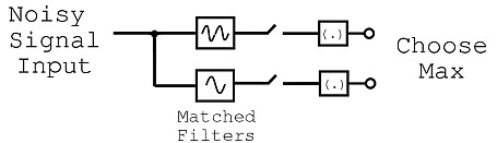
Block diagram of matched filter detector.
Figure 13.14 basically shows that our noisy signal will be passed in (we will assume that it passes in one "bit" at a time) and this signal will be split and passed to two different matched filter detectors. Each one will compare the noisy, received signal to one of the two codes we defined for '1' and '0.' Then this value will be passed on and whichever value is higher (i.e. whichever FSK code signal the noisy signal most resembles) will be the value that the receiver takes. For example, the first bit that will be sent through will be a '1' so the upper level of the block diagram will have a higher value, thus denoting that a '1' was sent by the signal, even though the signal may appear very noisy and distorted.
The interactive example below supposes that our transmitter sends 1000 bits, plotting how many of those bits are received and interpreted correctly as either 1s and 0s, and also keeps a tally of how many are accidentally misinterpreted. You can play around with the distance between the energy of the "1" and the "0" (discriminability), the degree of noise present in the channel, and the location of the criterion (threshold) to get a feel for the basics of signal detection theory.
Example 13.4.
Let's use a matched filter to find the "0" bits in a simple signal.
Let's use the signal s 1(t) from example 1 to represent the bits. s 1(t) represents 0, while – s 1(t) represents 1.
0 ⇒ b = 1 ⇒ s 1(t) = s(t) for 0 ≤ t ≤ T
1 ⇒ b = -1 ⇒ s 2(t) = – (s(t)) for 0 ≤ t ≤ T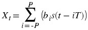
Figure 13.15.
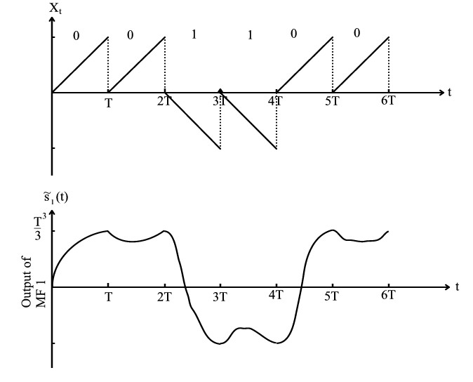
The matched filter output clearly shows the location of the "0" bits.
Radar
One of the first, and more intriguing forms of communication that used the matched filter concept was radar. A known electromagnetic signal is sent out by a transmitter at a target and reflected off of the target back to the sender with a time delay proportional to the distance between target and sender. This scaled, time-shifted signal is then convolved with the original template signal, and the time at which the output of this convolution is highest is noted.
This technology proved vital in the 1940s for the powers that possessed it. A short set of videos below shows the basics of how the technology works, its applications, and its impact in World War 2.
Figure 13.16. History of Radar
(This media type is not supported in this reader. Click to open media in browser.)
See the video in Figure 13.17 for an analysis of the same basic principle being applied to adaptive cruise control systems for the modern car.
Figure 13.17.
(This media type is not supported in this reader. Click to open media in browser.)
Video on radar-based adaptive cruise control from The Science Channel.
Matched Filter Demonstration
Figure 13.18.

Interact (when online) with a Mathematica CDF demonstrating the Matched Filter. To Download, right-click and save target as .cdf.
Matched Filter Summary
As can be seen, the matched filter detector is an important signal processing application, rich both in theoretical concepts and in practical applications. The matched filter supports a wide array of uses related to pattern recognition, including image detection, frequency shift keying demodulation, and radar signal interpretation. Despite this diversity of purpose, all matched filter applications operate in essentially the same way. Every member of some set of signals is compared to a target signal by evaluating the absolute value of the inner product of the the two signals after normalization. However, the signal sets and result interpretations are application specific.
Solutions to Exercises
Solution to Exercise 13.4.1. (Return to Exercise)
This algorithm is very simple and thus easy to code. However, it is susceptible to certain types of noise - for example, it would be difficult to find Waldo if his face was rotated, flipped, larger or smaller than expected, or distorted in some other way.
Chapter 14. Appendix A: Linear Algebra Overview
14.1. Basic Linear Algebra*
This brief tutorial on some key terms in linear algebra is not meant to replace or be very helpful to those of you trying to gain a deep insight into linear algebra. Rather, this brief introduction to some of the terms and ideas of linear algebra is meant to provide a little background to those trying to get a better understanding or learn about eigenvectors and eigenfunctions, which play a big role in deriving a few important ideas on Signals and Systems. The goal of these concepts will be to provide a background for signal decomposition and to lead up to the derivation of the Fourier Series.
Linear Independence
A set of vectors  are linearly independent if none of them can be written as a linear combination of the others.
Definition: Linearly Independent
For a given set of vectors,, they are linearly independent if
only when c 1 = c 2 = … = c n = 0
Example .
We are given the following two vectors:
These are not linearly independent as proven by the following statement, which, by inspection, can be seen to not adhere to the definition of linear independence stated above.
Another approach to reveal a vectors independence is by graphing the vectors. Looking at these two vectors geometrically (as in Figure 14.1), one can again prove that these vectors are not linearly independent.
Figure 14.1.
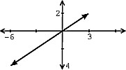
Graphical representation of two vectors that are not linearly independent.
Example 14.2.
We are given the following two vectors:
These are linearly independent since
only if c 1 = c 2 = 0 . Based on the definition, this proof shows that these vectors are indeed linearly independent. Again, we could also graph these two vectors (see Figure 14.2) to check for linear independence.
Figure 14.2.
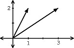
Graphical representation of two vectors that are linearly independent.
Exercise 14.1.1. (Go to Solution)
Are  linearly independent?


As we have seen in the two above examples, often times the independence of vectors can be easily seen through a graph. However this may not be as easy when we are given three or more vectors. Can you easily tell whether or not these vectors are independent from Figure 14.3. Probably not, which is why the method used in the above solution becomes important.
Figure 14.3.
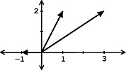
Plot of the three vectors. Can be shown that a linear combination exists among the three, and therefore they are not linear independent.
Hint
A set of m vectors in ℂn cannot be linearly independent if m > n .
Span
Definition: Span
The span of a set of vectorsis the set of vectors that can be written as a linear combination of


Example .
Given the vectorthe span of
is a line.
Example .
Given the vectors
the span of these vectors is ℂ2 .
Basis
Definition: Basis
A basis for ℂn is a set of vectors that: (1) spans ℂn and (2) is linearly independent.
Clearly, any set of n linearly independent vectors is a basis for ℂn .
Example 14.5.
We are given the following vectorwhere the 1 is always in the i th place and the remaining values are zero. Then the basis for ℂn is

Note
is called the standard basis.
Example 14.6.


is a basis for ℂ2 .
Figure 14.4.

Plot of basis for ℂ2
If  is a basis for ℂn
, then we can express any
x ∈ ℂn
as a linear combination of the b
i
's:
is a basis for ℂn
, then we can express any
x ∈ ℂn
as a linear combination of the b
i
's: 
Example 14.7.
Given the following vector,writing x in terms of
gives us
Exercise 14.1.2. (Go to Solution)
Try and write x in terms of  (defined in the previous example).
In the two basis examples above, x is the same vector in both cases, but we can express it in many different ways (we give only two out of many, many possibilities). You can take this even further by extending this idea of a basis to function spaces.
Note
As mentioned in the introduction, these concepts of linear algebra will help prepare you to understand the Fourier Series, which tells us that we can express periodic functions, f(t) , in terms of their basis functions, ⅇ ⅈ ω 0 n t .
(This media type is not supported in this reader. Click to open media in browser.)
Figure 14.5. Khan Lecture on Basis of a Subspace
(This media type is not supported in this reader. Click to open media in browser.)
video from Khan Academy, Basis of a Subspace - 20 min.
Solutions to Exercises
Solution to Exercise 14.1.1. (Return to Exercise)
By playing around with the vectors and doing a little trial and error, we will discover the following relationship:  Thus we have found a linear combination of these three vectors that equals zero without setting the coefficients equal to zero. Therefore, these vectors are not linearly independent!
Solution to Exercise 14.1.2. (Return to Exercise)
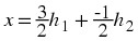
14.2. Eigenvectors and Eigenvalues*
In this section, our linear systems will be n×n matrices of complex numbers. For a little background into some of the concepts that this module is based on, refer to the basics of linear algebra.
Eigenvectors and Eigenvalues
Let A be an n×n matrix, where A is a linear operator on vectors in ℂn . Ax = b where x and b are n×1 vectors (Figure 14.6).
Figure 14.6.
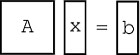
(a)
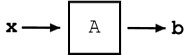
(b)
Illustration of linear system and vectors.
Definition: eigenvector
An eigenvector of A is a vector v ∈ ℂn such that
(14.1)Av = λv
where λ is called the corresponding eigenvalue. A only changes the length of v , not its direction.
Graphical Model
Through Figure 14.7 and Figure 14.8, let us look at the difference between Equation and Equation 14.1.
Figure 14.7.
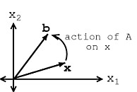
Represents Equation, Ax = b .
If v is an eigenvector of A , then only its length changes. See Figure 14.8 and notice how our vector's length is simply scaled by our variable, λ , called the eigenvalue:
Figure 14.8.
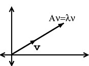
Represents Equation 14.1, Av = λv .
Note
When dealing with a matrix A , eigenvectors are the simplest possible vectors to operate on.
Examples
Exercise 14.2.1. (Go to Solution)
From inspection and understanding of eigenvectors, find the two eigenvectors,  and
and  , of
, of  Also, what are the corresponding eigenvalues, λ
1 and λ
2 ? Do not worry if you are having problems seeing these values from the information given so far, we will look at more rigorous ways to find these values soon.
Also, what are the corresponding eigenvalues, λ
1 and λ
2 ? Do not worry if you are having problems seeing these values from the information given so far, we will look at more rigorous ways to find these values soon.
Exercise 14.2.2. (Go to Solution)
Show that these two vectors, 
 are eigenvectors of A , where
  . Also, find the corresponding eigenvalues.
Figure 14.9. Khan Lecture on Eigenvectors
(This media type is not supported in this reader. Click to open media in browser.)
video from Khan Academy - Introduction to Eigenvectors and Eigenvalues - 7:43 min.
Calculating Eigenvalues and Eigenvectors
In the above examples, we relied on your understanding of the definition and on some basic observations to find and prove the values of the eigenvectors and eigenvalues. However, as you can probably tell, finding these values will not always be that easy. Below, we walk through a rigorous and mathematical approach at calculating the eigenvalues and eigenvectors of a matrix.
Finding Eigenvalues
Find λ ∈ ℂ such that v ≠ 0 , where 0 is the "zero vector." We will start with Equation 14.1, and then work our way down until we find a way to explicitly calculate λ . Av = λv Av − λv = 0 (A − λI)v = 0 In the previous step, we used the fact that λv = λIv where I is the identity matrix.  So, A − λI is just a new matrix.
Example 14.8.
Given the following matrix, A , then we can find our new matrix, A − λI .

If (A − λI)v = 0 for some v ≠ 0 , then A − λI is not invertible. This means: det(A − λI) = 0 This determinant (shown directly above) turns out to be a polynomial expression (of order n ). Look at the examples below to see what this means.
Example 14.9.
Starting with matrix A (shown below), we will find the polynomial expression, where our eigenvalues will be the dependent variable.


Example 14.10.
Starting with matrix A (shown below), we will find the polynomial expression, where our eigenvalues will be the dependent variable.
det(A − λI) = λ 2 − (a 11 + a 22)λ − a 21 a 12 + a 11 a 22
If you have not already noticed it, calculating the eigenvalues is equivalent to calculating the roots of det(A − λI) = c n λ n + c n − 1 λ n − 1 + … + c 1 λ + c 0 = 0
Conclusion
Therefore, by simply using calculus to solve for the roots of our polynomial we can easily find the eigenvalues of our matrix.
Finding Eigenvectors
Given an eigenvalue, λ
i
, the associated eigenvectors are given by Av = λ
i
v 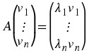 set of n equations with n unknowns. Simply solve the n equations to find the eigenvectors.
Figure 14.10. Khan Lecture on Deriving Eigenvectors and Eigenvalues
(This media type is not supported in this reader. Click to open media in browser.)
video from Khan Academy - Example Deriving Eignevectors and Eigenvalues - 5:39 min.
Main Point
Say the eigenvectors of A ,  , span ℂn
, meaning
, span ℂn
, meaning  are linearly independent and we can write any x ∈ ℂn
as
are linearly independent and we can write any x ∈ ℂn
as 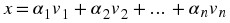 where
where  . All that we are doing is rewriting x in terms of eigenvectors of A . Then,

 Therefore we can write,
 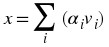 and this leads us to the following depicted system:
Figure 14.11.

Depiction of system where we break our vector, x , into a sum of its eigenvectors.
where in Figure 14.11 we have, 
Main Point
By breaking up a vector, x , into a combination of eigenvectors, the calculation of Ax is broken into "easy to swallow" pieces.
Practice Problem
Exercise 14.2.3. (Go to Solution)
For the following matrix, A and vector, x , solve for their product. Try solving it using two different methods: directly and using eigenvectors. 

(This media type is not supported in this reader. Click to open media in browser.)
Solutions to Exercises
Solution to Exercise 14.2.1. (Return to Exercise)
The eigenvectors you found should be: 
 And the corresponding eigenvalues are λ
1 = 3 λ
2 = -1
And the corresponding eigenvalues are λ
1 = 3 λ
2 = -1
Solution to Exercise 14.2.2. (Return to Exercise)
In order to prove that these two vectors are eigenvectors, we will show that these statements meet the requirements stated in the definition. 
 These results show us that A only scales the two vectors (i.e. changes their length) and thus it proves that Equation 14.1 holds true for the following two eigenvalues that you were asked to find: λ
1 = 2 λ
2 = 4 If you need more convincing, then one could also easily graph the vectors and their corresponding product with A to see that the results are merely scaled versions of our original vectors,
These results show us that A only scales the two vectors (i.e. changes their length) and thus it proves that Equation 14.1 holds true for the following two eigenvalues that you were asked to find: λ
1 = 2 λ
2 = 4 If you need more convincing, then one could also easily graph the vectors and their corresponding product with A to see that the results are merely scaled versions of our original vectors,  and
and  .
.
Solution to Exercise 14.2.3. (Return to Exercise)
Direct Method (use basic matrix multiplication)  Eigenvectors (use the eigenvectors and eigenvalues we found earlier for this same matrix)
 λ
1 = 2 λ
2 = 4 As shown in Equation, we want to represent x as a sum of its scaled eigenvectors. For this case, we have:
λ
1 = 2 λ
2 = 4 As shown in Equation, we want to represent x as a sum of its scaled eigenvectors. For this case, we have: 

 Therefore, we have
  Notice that this method using eigenvectors required no matrix multiplication. This may have seemed more complicated here, but just imagine A being really big, or even just a few dimensions larger!
14.3. Matrix Diagonalization*
From our understanding of eigenvalues and eigenvectors we have discovered several things about our operator matrix, A . We know that if the eigenvectors of A span ℂn
and we know how to express any vector x in terms of  , then we have the operator A all figured out. If we have A acting on x , then this is equal to A acting on the combinations of eigenvectors. Which we know proves to be fairly easy!
We are still left with two questions that need to be addressed:
When do the eigenvectors
 of A span ℂn
(assuming
of A span ℂn
(assuming  are linearly independent)?
 How do we express a given vector x in terms of
 ?
?
Answer to Question #1
Question #1
When do the eigenvectorsof A span ℂn ?
If A has n distinct eigenvalues λ
i
≠ λ
j
, i ≠ j where i and j are integers, then A has n linearly independent eigenvectors  which then span ℂn
.
which then span ℂn
.
Note
The proof of this statement is not very hard, but is not really interesting enough to include here. If you wish to research this idea further, read Strang, G., "Linear Algebra and its Application" for the proof.
Furthermore, n distinct eigenvalues means det(A − λI) = c n λ n + c n − 1 λ n − 1 + … + c 1 λ + c 0 = 0 has n distinct roots.
Answer to Question #2
Question #2
How do we express a given vector x in terms of?
We want to find  such that
  In order to find this set of variables, we will begin by collecting the vectors
  as columns in a n×n matrix V .
  Now Equation becomes
  or x = Vα which gives us an easy form to solve for our variables in question, α : α = V
-1
x Note that V is invertible since it has n linearly independent columns.
or x = Vα which gives us an easy form to solve for our variables in question, α : α = V
-1
x Note that V is invertible since it has n linearly independent columns.
Aside
Let us recall our knowledge of functions and their basis and examine the role of V . x = Vα  where α is just x expressed in a different basis:
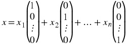
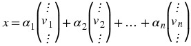 V transforms
x from the standard basis to the basis
V transforms
x from the standard basis to the basis 
Matrix Diagonalization and Output
We can also use the vectors  to represent the output, b , of a system:

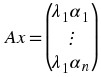 Ax = VΛα Ax = V
Λ
V
-1
x where Λ is the matrix with the eigenvalues down the diagonal:
Ax = VΛα Ax = V
Λ
V
-1
x where Λ is the matrix with the eigenvalues down the diagonal: 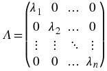 Finally, we can cancel out the x and are left with a final equation for A : A = V
Λ
V
-1
Finally, we can cancel out the x and are left with a final equation for A : A = V
Λ
V
-1
Interpretation
For our interpretation, recall our key formulas: α = V
-1
x  We can interpret operating on x with A as:
 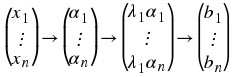 where the three steps (arrows) in the above illustration represent the following three operations:
Transform x using V -1 , which yields α
Multiplication by Λ
Inverse transform using V , which gives us b
This is the paradigm we will use for LTI systems!
Figure 14.12.

Simple illustration of LTI system!
(This media type is not supported in this reader. Click to open media in browser.)
14.4. Eigen-stuff in a Nutshell*
A Matrix and its Eigenvector
The reason we are stressing eigenvectors and their importance is because the action of a matrix A on one of its eigenvectors v is
extremely easy (and fast) to calculate Av = λv just multiply v by λ .
easy to interpret: A just scales v , keeping its direction constant and only altering the vector's length.
If only every vector were an eigenvector of A ....
Using Eigenvectors' Span
Of course, not every vector can be ... BUT ... For certain matrices (including ones with distinct eigenvalues, λ 's), their eigenvectors span ℂn
, meaning that for any
x ∈ ℂn
, we can find  such that:
  Given Equation, we can rewrite Ax = b . This equation is modeled in our LTI system pictured below:
Figure 14.13.
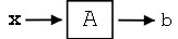
LTI System.

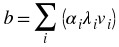 The LTI system above represents our Equation. Below is an illustration of the steps taken to go from x to b . x → (α = V
-1
x) → (Λ
V
-1
x) → V
Λ
V
-1
x = b where the three steps (arrows) in the above illustration represent the following three operations:
The LTI system above represents our Equation. Below is an illustration of the steps taken to go from x to b . x → (α = V
-1
x) → (Λ
V
-1
x) → V
Λ
V
-1
x = b where the three steps (arrows) in the above illustration represent the following three operations:
Transform x using V -1 - yields α
Action of A in new basis - a multiplication by Λ
Translate back to old basis - inverse transform using a multiplication by V , which gives us b
14.5. Eigenfunctions of LTI Systems*
Introduction
Hopefully you are familiar with the notion of the eigenvectors of a "matrix system," if not they do a quick review of eigen-stuff. We can develop the same ideas for LTI systems acting on signals. A linear time invariant (LTI) system ℋ operating on a continuous input f(t) to produce continuous time output y(t) ℋ[f(t)] = y(t)
Figure 14.14.

ℋ[f(t)] = y(t) . f and t are continuous time (CT) signals and ℋ is an LTI operator.
is mathematically analogous to an N xN matrix A operating on a vector x ∈ ℂ N to produce another vector b ∈ ℂ N (see Matrices and LTI Systems for an overview). Ax = b
Figure 14.15.
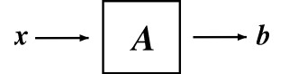
Ax = b where x and b are in ℂ N and A is an N x N matrix.
Just as an eigenvector of A is a v ∈ ℂ N such that Av = λv , λ ∈ ℂ ,
Figure 14.16.
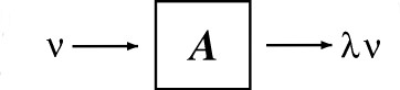
Av = λv where v ∈ ℂ N is an eigenvector of A .
we can define an eigenfunction (or eigensignal) of an LTI system ℋ to be a signal f(t) such that ℋ[f(t)] = λ f(t) , λ ∈ ℂ
Figure 14.17.
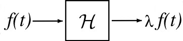
ℋ[f(t)] = λ f(t) where f is an eigenfunction of ℋ .
Eigenfunctions are the simplest possible signals for ℋ to operate on: to calculate the output, we simply multiply the input by a complex number λ .
Eigenfunctions of any LTI System
The class of LTI systems has a set of eigenfunctions in common: the complex exponentials ⅇ st , s ∈ ℂ are eigenfunctions for all LTI systems. ℋ[ⅇ st ] = λ s ⅇ st
Figure 14.18.
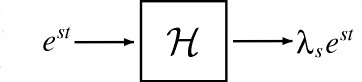
ℋ[ⅇ st ] = λ s ⅇ st where ℋ is an LTI system.
Note
While {ⅇ st , s ∈ ℂ } are always eigenfunctions of an LTI system, they are not necessarily the only eigenfunctions.
We can prove Equation by expressing the output as a convolution of the input ⅇ
st
and the impulse response
h(t) of ℋ : 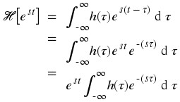 Since the expression on the right hand side does not depend on t , it is a constant, λ
s
. Therefore ℋ[ⅇ
st
] = λ
s
ⅇ
st
The eigenvalue λ
s
is a complex number that depends on the exponent s and, of course, the system ℋ . To make these dependencies explicit, we will use the notation H(s) ≡ λ
s
.
Since the expression on the right hand side does not depend on t , it is a constant, λ
s
. Therefore ℋ[ⅇ
st
] = λ
s
ⅇ
st
The eigenvalue λ
s
is a complex number that depends on the exponent s and, of course, the system ℋ . To make these dependencies explicit, we will use the notation H(s) ≡ λ
s
.
Figure 14.19.
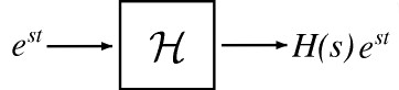
ⅇ st is the eigenfunction and H(s) are the eigenvalues.
Since the action of an LTI operator on its eigenfunctions ⅇ st is easy to calculate and interpret, it is convenient to represent an arbitrary signal f(t) as a linear combination of complex exponentials. The Fourier series gives us this representation for periodic continuous time signals, while the (slightly more complicated) Fourier transform lets us expand arbitrary continuous time signals.
Chapter 15. Appendix B: Hilbert Spaces Overview
15.1. Fields and Complex Numbers*
Fields
In order to propely discuss the concept of vector spaces in linear algebra, it is necessary to develop the notion of a set of “scalars” by which we allow a vector to be multiplied. A framework within which our concept of real numbers would fit is desireable. Thus, we would like a set with two associative, commutative operations (like standard addition and multiplication) and a notion of their inverse operations (like subtraction and division). The mathematical algebraic construct that addresses this idea is the field. A field (S, + , * ) is a set S together with two binary operations + and * such that the following properties are satisfied.
Closure of S under + : For every x,y ∈ S , x + y ∈ S .
Associativity of S under + : For every x,y,z ∈ S , (x + y) + z = x + (y + z).
Existence of + identity element: There is a e + ∈ S such that for every x ∈ S , e + + x = x + e + = x .
Existence of + inverse elements: For every x ∈ S there is a y ∈ S such that x + y = y + x = e + .
Commutativity of S under + : For every x,y ∈ S , x + y = y + x .
Closure of S under * : For every x,y ∈ S , x * y ∈ S .
Associativity of S under * : For every x,y,z ∈ S , (x * y) * z = x * (y * z).
Existence of * identity element: There is a e * ∈ S such that for every x ∈ S , e * + x = x + e * = x .
Existence of * inverse elements: For every x ∈ S with x ≠ e + there is a y ∈ S such that x * y = y * x = e * .
Commutativity of S under * : For every x,y ∈ S , x * y = y * x .
Distributivity of * over + : For every x,y,z ∈ S , x * (y + z) = x y + x z .
While this definition is quite general, the two fields used most often in signal processing, at least within the scope of this course, are the real numbers and the complex numbers, each with their typical addition and multiplication operations.
The Complex Field
The reader is undoubtedly already sufficiently familiar with the real numbers with the typical addition and multiplication operations. However, the field of complex numbers with the typical addition and multiplication operations may be unfamiliar to some. For that reason and its importance to signal processing, it merits a brief explanation here.
Definitions
The notion of the square root of -1 originated with the quadratic formula: the solution of certain quadratic equations mathematically exists only if the so-called imaginary quantity  could be defined. Euler first used i for the imaginary unit but that notation did not take hold until roughly Ampère's time. Ampère used the symbol i to denote current (intensité de current). It wasn't until the twentieth century that the importance of complex numbers to circuit theory became evident. By then, using i for current was entrenched and electrical engineers now choose j for writing complex numbers.
An imaginary number has the form  . A complex number, z , consists of the ordered pair (a ,b ), a is the real component and b is the imaginary component (the j is suppressed because the imaginary component of the pair is always in the second position). The imaginary number jb equals (0,b ). Note that a and b are real-valued numbers.
Figure 15.1 shows that we can locate a complex number in what we call the complex plane. Here, a , the real part, is the x -coordinate and b , the imaginary part, is the y -coordinate.
Figure 15.1. The Complex Plane
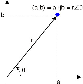
A complex number is an ordered pair (a ,b ) that can be regarded as coordinates in the plane. Complex numbers can also be expressed in polar coordinates as r∠θ .
From analytic geometry, we know that locations in the plane can be expressed as the sum of vectors, with the vectors corresponding to the x and y directions. Consequently, a complex number z can be expressed as the (vector) sum z = a + jb where j indicates the y -coordinate. This representation is known as the Cartesian form of z . An imaginary number can't be numerically added to a real number; rather, this notation for a complex number represents vector addition, but it provides a convenient notation when we perform arithmetic manipulations.
The real part of the complex number z = a + jb , written as Re(z) , equals a . We consider the real part as a function that works by selecting that component of a complex number not multiplied by j . The imaginary part of z , Im(z) , equals b : that part of a complex number that is multiplied by j . Again, both the real and imaginary parts of a complex number are real-valued.
The complex conjugate of z , written as  , has the same real part as z but an imaginary part of the opposite sign.
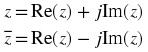
Using Cartesian notation, the following properties easily follow.
If we add two complex numbers, the real part of the result equals the sum of the real parts and the imaginary part equals the sum of the imaginary parts. This property follows from the laws of vector addition. a 1 + j b 1 + a 2 + j b 2 = a 1 + a 2 + j(b 1 + b 2) In this way, the real and imaginary parts remain separate.
The product of j and a real number is an imaginary number: ja . The product of j and an imaginary number is a real number: j(jb) = – b because j 2 = – 1 . Consequently, multiplying a complex number by j rotates the number's position by 90 degrees.
Exercise 15.1.1. (Go to Solution)
Use the definition of addition to show that the real and imaginary parts can be expressed as a sum/difference of a complex number and its conjugate. 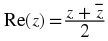 and
and 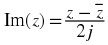 .
.
Complex numbers can also be expressed in an alternate form, polar form, which we will find quite useful. Polar form arises arises from the geometric interpretation of complex numbers. The Cartesian form of a complex number can be re-written as 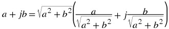 By forming a right triangle having sides a and b , we see that the real and imaginary parts correspond to the cosine and sine of the triangle's base angle. We thus obtain the polar form for complex numbers.
 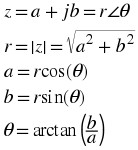 The quantity r is known as the magnitude of the complex number z , and is frequently written as |z| . The quantity θ is the complex number's angle. In using the arc-tangent formula to find the angle, we must take into account the quadrant in which the complex number lies.
Exercise 15.1.2. (Go to Solution)
Convert 3 − 2j to polar form.
Euler's Formula
Surprisingly, the polar form of a complex number z can be expressed mathematically as z = r
ⅇ
jθ
To show this result, we use Euler's relations that express exponentials with imaginary arguments in terms of trigonometric functions. ⅇ
jθ
= cos(θ) + jsin(θ) 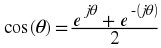
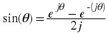 The first of these is easily derived from the Taylor's series for the exponential.
 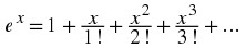 Substituting jθ for x , we find that
 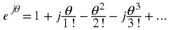 because j
2 = -1 , j
3 = – j , and j
4 = 1 . Grouping separately the real-valued terms and the imaginary-valued ones,
because j
2 = -1 , j
3 = – j , and j
4 = 1 . Grouping separately the real-valued terms and the imaginary-valued ones, 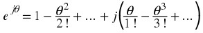 The real-valued terms correspond to the Taylor's series for cos(θ) , the imaginary ones to sin(θ) , and Euler's first relation results. The remaining relations are easily derived from the first. Because of ???, we see that multiplying the exponential in Equation by a real constant corresponds to setting the radius of the complex number by the constant.
Calculating with Complex Numbers
Adding and subtracting complex numbers expressed in Cartesian form is quite easy: You add (subtract) the real parts and imaginary parts separately. (z
1 ± z
2) = (a
1 ± a
2) + j(b
1 ± b
2) To multiply two complex numbers in Cartesian form is not quite as easy, but follows directly from following the usual rules of arithmetic. 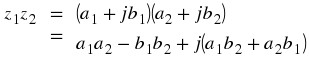 Note that we are, in a sense, multiplying two vectors to obtain another vector. Complex arithmetic provides a unique way of defining vector multiplication.
Exercise 15.1.3. (Go to Solution)
What is the product of a complex number and its conjugate?
Division requires mathematical manipulation. We convert the division problem into a multiplication problem by multiplying both the numerator and denominator by the conjugate of the denominator.  Because the final result is so complicated, it's best to remember how to perform division—multiplying numerator and denominator by the complex conjugate of the denominator—than trying to remember the final result.
The properties of the exponential make calculating the product and ratio of two complex numbers much simpler when the numbers are expressed in polar form. 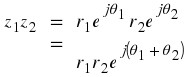
 To multiply, the radius equals the product of the radii and the angle the sum of the angles. To divide, the radius equals the ratio of the radii and the angle the difference of the angles. When the original complex numbers are in Cartesian form, it's usually worth translating into polar form, then performing the multiplication or division (especially in the case of the latter). Addition and subtraction of polar forms amounts to converting to Cartesian form, performing the arithmetic operation, and converting back to polar form.
Solutions to Exercises
Solution to Exercise 15.1.1. (Return to Exercise)
 . Similarly,
Solution to Exercise 15.1.2. (Return to Exercise)
To convert 3 − 2j to polar form, we first locate the number in the complex plane in the fourth quadrant. The distance from the origin to the complex number is the magnitude r , which equals  . The angle equals
  or -0.588 radians ( – 33.7 degrees). The final answer is
  degrees.
Solution to Exercise 15.1.3. (Return to Exercise)
 . Thus,
  .
.
15.2. Vector Spaces*
Introduction
Definition: Vector space
A vector space S is a collection of "vectors" such that (1) if f 1 ∈ S ⇒ α f 1 ∈ S for all scalars α (where α ∈ ℝ , α ∈ ℂ , or some other field) and (2) if f 1 ∈ S , f 2 ∈ S , then f 1 + f 2 ∈ S
To define an vector space, we need
A set of things called "vectors" (X )
A set of things called "scalars" that form a field (A )
A vector addition operation ( + )
A scalar multiplication operation (* )
The operations need to have all the properties of given below. Closure is usually the most important to show.
Vector Spaces
If the scalars α are real, S is called a real vector space.
If the scalars α are complex, S is called a complex vector space.
If the "vectors" in S are functions of a continuous variable, we sometimes call S a linear function space
Properties
We define a set V to be a vector space if
x + y = y + x for each x and y in V
x + (y + z) = (x + y) + z for each x , y , and z in V
There is a unique "zero vector" such that x + 0 = x for each x in V (0 is the field additive identity)
For each x in V there is a unique vector – x such that x + ( – x) = 0
1x = x (1 is the field multiplicative identity)
 for each x in V and c
1 and c
2 in ℂ
for each x in V and c
1 and c
2 in ℂ c(x + y) = cx + cy for each x and y in V and c in ℂ
(c 1 + c 2)x = c 1 x + c 2 x for each x in V and c 1 and c 2 in ℂ
Examples
ℝn = real vector space
ℂn = complex vector space
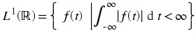 is a vector space
 L ∞(ℝ) = {f(t)| f ( t ) is bounded } is a vector space
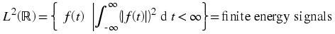 is a vector space
ℓ 1(ℤ) , ℓ 2(ℤ) , ℓ ∞(ℤ) are vector spaces
The collection of functions piecewise constant between the integers is a vector space
Figure 15.2.
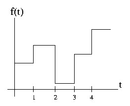
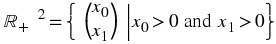 is not a vector space.
  , but
, but 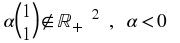
D = {z ∈ ℂ , |z| ≤ 1 } is not a vector space. z 1 = 1 ∈ D , z 2 = ⅈ ∈ D , but z 1 + z 2 ∉ D ,
Note
Vector spaces can be collections of functions, collections of sequences, as well as collections of traditional vectors (i.e. finite lists of numbers)
15.3. Norms*
Introduction
This module will explain norms, a mathematical concept that provides a notion of the size of a vector. Specifically, the general definition of a norm will be discussed and discrete time signal norms will be presented.
Norms
The norm of a vector is a real number that represents the "size" of the vector.
Example 15.1.
In ℝ2 , we can define a norm to be a vectors geometric length.
Figure 15.3.
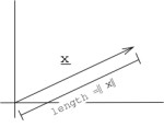
x = (x 0, x 1)T , norm
Mathematically, a norm ∥ · ∥ is just a function (taking a vector and returning a real number) that satisfies three rules.
To be a norm, ∥ · ∥ must satisfy:
the norm of every vector is positive ∥ x ∥ > 0 , x ∈ S
scaling a vector scales the norm by the same amount ∥ αx ∥ = |α| ∥ x ∥ for all vectors x and scalars α
Triangle Property: ∥ x + y ∥ ≤ ∥ x ∥ + ∥ y ∥ for all vectors x , y . "The "size" of the sum of two vectors is less than or equal to the sum of their sizes"
A vector space with a well defined norm is called a normed vector space or normed linear space.
Examples
Example 15.2.
ℝn (or ℂn ),,
, ℝn with this norm is called
.
Figure 15.4.
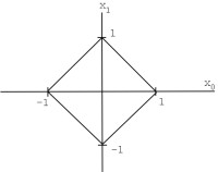
Collection of all x ∈ ℝ2 with ∥ x ∥ 1 = 1
Example 15.3.
ℝn (or ℂn ), with norm, ℝn is called
(the usual "Euclidean"norm).
Figure 15.5.
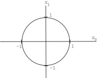
Collection of all x ∈ ℝ2 with ∥ x ∥ 2 = 1
Example 15.4.
ℝn (or ℂn , with normis called
Figure 15.6.
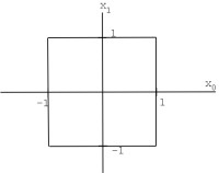
x ∈ ℝ2 with ∥ x ∥ ∞ = 1
Spaces of Sequences and Functions
We can define similar norms for spaces of sequences and functions.
Discrete time signals = sequences of numbers x[n] = {…, x -2, x -1, x 0, x 1, x 2, …}
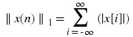 ,
, 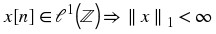
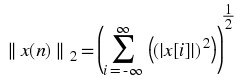 ,
, 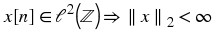
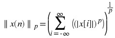 ,
, 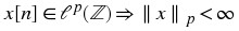
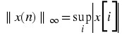 ,
, 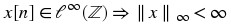
For continuous time functions:
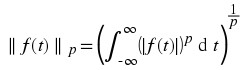 ,
, 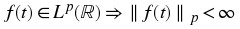
(On the interval)
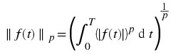 ,
, 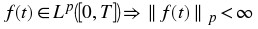
15.4. Inner Products*
Definition: Inner Product
You may have run across inner products, also called dot products, on ℝn before in some of your math or science courses. If not, we define the inner product as follows, given we have some x ∈ ℝn and y ∈ ℝn
Definition: standard inner product
The standard inner product is defined mathematically as: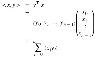
Inner Product in 2-D
If we have x ∈ ℝ2 and y ∈ ℝ2 , then we can write the inner product as < x,y > = ∥ x ∥ ∥ y ∥ cos(θ) where θ is the angle between x and y .
Figure 15.7.
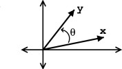
General plot of vectors and angle referred to in above equations.
Geometrically, the inner product tells us about the strength of x in the direction of y .
Example 15.5.
For example, if ∥ x ∥ = 1 , then < x,y > = ∥ y ∥ cos(θ)
Figure 15.8.
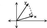
Plot of two vectors from above example.
The following characteristics are revealed by the inner product:
< x,y > measures the length of the projection of y onto x .
< x,y > is maximum (for given ∥ x ∥ , ∥ y ∥ ) when x and y are in the same direction ( θ = 0 ⇒ cos(θ) = 1 ).
< x,y > is zero when cos(θ) = 0 ⇒ θ = 90° , i.e. x and y are orthogonal.
Inner Product Rules
In general, an inner product on a complex vector space is just a function (taking two vectors and returning a complex number) that satisfies certain rules:
Conjugate Symmetry:
Scaling: < αx,y > = α < x,y >
Additivity: < x + y,z > = < x,z > + < y,z >
"Positivity": < x,x > > 0 , x ≠ 0
Definition: orthogonal
We say that x and y are orthogonal if: < x,y > = 0
(This media type is not supported in this reader. Click to open media in browser.)
15.5. Hilbert Spaces*
Hilbert Spaces
A vector space S with a valid inner product defined on it is called an inner product space, which is also a normed linear space. A Hilbert space is an inner product space that is complete with respect to the norm defined using the inner product. Hilbert spaces are named after David Hilbert, who developed this idea through his studies of integral equations. We define our valid norm using the inner product as:  Hilbert spaces are useful in studying and generalizing the concepts of Fourier expansion, Fourier transforms, and are very important to the study of quantum mechanics. Hilbert spaces are studied under the functional analysis branch of mathematics.
Examples of Hilbert Spaces
Below we will list a few examples of Hilbert spaces. You can verify that these are valid inner products at home.
For ℂn ,
Space of finite energy complex functions: L 2(ℝ)

Space of square-summable sequences: ℓ 2(ℤ)
15.6. Cauchy-Schwarz Inequality*
Introduction
Any treatment of linear algebra as relates to signal processing would not be complete without a discussion of the Cauchy-Schwarz ineqaulity, a relation that enables a wide array of signal procesing applications related to pattern matching through a method called the matched filter. Recall that in standard Euclidean space, the angle θ between two vectors x,y is given by
(15.1)
Since cos(θ) ≤ 1, it follows that
(15.2) | 〈 x , y 〉 | 2 ≤ 〈 x , x 〉 〈 y , y 〉 .
Furthermore, equality holds if and only if cos(θ) = 0, implying that
(15.3) | 〈 x , y 〉 | 2 = 〈 x , x 〉 〈 y , y 〉
if and only if y = a x for some real a . This relation can be extended to all inner product spaces over a real or complex field and is known as the Cauchy-Schwarz inequality, which is of great importance to the study of signals.
The Cauchy-Schwarz Inequality
Statement of the Cauchy-Schwarz Inequality
The general statement of the Cauchy-Schwarz inequality mirrors the intuition for standard Euclidean space. Let V be an inner product space over the field of complex numbers C with inner product 〈 · , · 〉. For every pair of vectors x,y ∈ V the inequality
(15.4) | 〈 x , y 〉 | 2 ≤ 〈 x , x 〉 〈 y , y 〉
holds. Furthermore, the equality
(15.5) | 〈 x , y 〉 | 2 = 〈 x , x 〉 〈 y , y 〉
holds if and only if y = a x for some a ∈ C. That is, equality holds if and only if x and y are linearly dependent.
Proof of the Cauchy-Schwarz Inequality
Let V be a vector space over the real or complex field F , and let x,y ∈ V be given. In order to prove the Cauchy-Schwarz inequality, it will first be proven that |〈x,y〉|2 = 〈x,x〉〈y,y〉 if y = a x for some a ∈ F . It will then be shown that |〈x,y〉|2 < 〈x,x〉〈y,y〉 if y ≠ a x for all a ∈ F .
Consider the case in which y = a x for some a ∈ F . From the properties of inner products, it is clear that
(15.6)

Hence, it follows that
(15.7)
Similarly, it is clear that
(15.8)
Thus, it is proven that |〈x,y〉|2 = 〈x,x〉〈y,y〉 if x = a y for some a ∈ F .
Next, consider the case in which y ≠ a x for all a ∈ F , which implies that y ≠ 0 so 〈y,y〉 ≠ 0. Thus, it follows by the properties of inner products that, for all a ∈ F , 〈x – a y,x – a y〉 > 0. This can be expanded using the properties of inner products to the expression
(15.9)
Choosing  ,
,
(15.10)
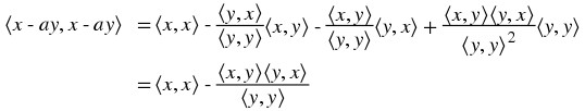
Hence, it follows that 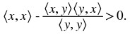 Consequently,
 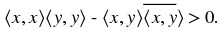 Thus, it can be concluded that |〈x,y〉|2 < 〈x,x〉〈y,y〉 if y ≠ a
x for all a ∈ F .
Thus, it can be concluded that |〈x,y〉|2 < 〈x,x〉〈y,y〉 if y ≠ a
x for all a ∈ F .
Therefore, the inequality
(15.11) | 〈 x , y 〉 | 2 ≤ 〈 x , x 〉 〈 y , y 〉
holds for all x,y ∈ V , and equality
(15.12) | 〈 x , y 〉 | 2 = 〈 x , x 〉 〈 y , y 〉
holds if and only if y = a x for some a ∈ F .
Additional Mathematical Implications
Consider the maximization of  where the norm || · || = 〈 · , · 〉 is induced by the inner product. By the Cauchy-Schwarz inequality, we know that
  and that
 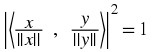 if and only if
  for some a ∈ C. Hence,
  attains a maximum where
  for some a ∈ C. Thus, collecting the scalar variables,
  attains a maximum where y = a
x . This result will be particulaly useful in developing the matched filter detector techniques.
attains a maximum where y = a
x . This result will be particulaly useful in developing the matched filter detector techniques.
Matched Filter Detector
Background Concepts
A great many applications in signal processing, image processing, and beyond involve determining the presence and location of a target signal within some other signal. A radar system, for example, searches for copies of a transmitted radar pulse in order to determine the presence of and distance to reflective objects such as building or aircraft. A communication system searches for copies of waveforms representing digital 0s and 1s in order to receive a message.
As has already been shown, the expression  attains its upper bound, which is 1, when y = a
x for some scalar a in a real or complex field. The lower bound, which is 0, is attained when x and y are orthogonal. In informal intuition, this means that the expression is maximized when the vectors x and y have the same shape or pattern and minimized when x and y are very different. A pair of vectors with similar but unequal shapes or patterns will produce relatively large value of the expression less than 1, and a pair of vectors with very different but not orthogonal shapes or patterns will produce relatively small values of the expression greater than 0. Thus, the above expression carries with it a notion of the degree to which two signals are “alike”, the magnitude of the normalized correlation between the signals in the case of the standard inner products.
attains its upper bound, which is 1, when y = a
x for some scalar a in a real or complex field. The lower bound, which is 0, is attained when x and y are orthogonal. In informal intuition, this means that the expression is maximized when the vectors x and y have the same shape or pattern and minimized when x and y are very different. A pair of vectors with similar but unequal shapes or patterns will produce relatively large value of the expression less than 1, and a pair of vectors with very different but not orthogonal shapes or patterns will produce relatively small values of the expression greater than 0. Thus, the above expression carries with it a notion of the degree to which two signals are “alike”, the magnitude of the normalized correlation between the signals in the case of the standard inner products.
This concept can be extremely useful. For instance consider a situation in which we wish to determine which signal, if any, from a set X of signals most resembles a particular signal y . In order to accomplish this, we might evaluate the above expression for every signal x ∈ X , choosing the one that results in maxima provided that those maxima are above some threshold of “likeness”. This is the idea behind the matched filter detector, which compares a set of signals against a target signal using the above expression in order to determine which among them are most like the target signal. For a detailed treatment of the applications of the matched filter detector see the liked module.
Signal Comparison
The simplest variant of the matched filter detector scheme would be to find the member signal in a set X of signals that most closely matches a target signal y . Thus, for every x ∈ X we wish to evaluate
(15.13)
in order to compare every member of X to the target signal y . Since the member of X which most closely matches the target signal y is desired, ultimately we wish to evaluate
(15.14)
Note that the target signal does not technically need to be normalized to produce a maximum, but gives the desirable property that m(x,y) is bounded to [0,1].
The element x m ∈ X that produces the maximum value of m(x,y) is not necessarily unique, so there may be more than one matching signal in X . Additionally, the signal x m ∈ X producing the maximum value of m(x,y) may not produce a very large value of m(x,y) and thus not be very much like the target signal y . Hence, another matched filter scheme might identify the argument producing the maximum but only above a certain threshold, returning no matching signals in X if the maximum is below the threshold. There also may be a signal x ∈ X that produces a large value of m(x,y) and thus has a high degree of “likeness” to y but does not produce the maximum value of m(x,y). Thus, yet another matched filter scheme might identify all signals in X producing local maxima that are above a certain threshold.
Example 15.6.
For example, consider the target signal given in Figure 15.9 and the set of two signals given in Figure 15.10. By inspection, it is clear that the signal g 2 is most like the target signal f . However, to make that conclusion mathematically, we use the matched filter detector with the L 2 inner product. If we were to actually make the necessary computations, we would first normalize each signal and then compute the necessary inner products in order to compare the signals in X with the target signal f . We would notice that the absolute value of the inner product for g 2 with f when normalized is greater than the absolute value of the inner product of g 1 with f when normalized, mathematically stated as
(15.15)
Figure 15.9. Template Signal
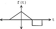
We wish to find a match for this target signal in the set of signals below.
Figure 15.10. Candidate Signals
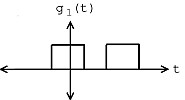
(a)

(b)
We wish to find a match for the above target signal in this set of signals.
Pattern Detection
A somewhat more involved matched filter detector scheme would involve attempting to match a target time limited signal y = f to a set of of time shifted and windowed versions of a single signal  indexed by R. The windowing funtion is given by
 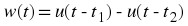 where
where  is the interval to which f is time limited. This scheme could be used to find portions of g that have the same shape as f . If the absolute value of the inner product of the normalized versions of f and w
S
t
g is large, which is the absolute value of the normalized correlation for standard inner products, then g has a high degree of “likeness” to f on the interval to which f is time limited but left shifted by t . Of course, if f is not time limited, it means that the entire signal has a high degree of “likeness” to f left shifted by t .
is the interval to which f is time limited. This scheme could be used to find portions of g that have the same shape as f . If the absolute value of the inner product of the normalized versions of f and w
S
t
g is large, which is the absolute value of the normalized correlation for standard inner products, then g has a high degree of “likeness” to f on the interval to which f is time limited but left shifted by t . Of course, if f is not time limited, it means that the entire signal has a high degree of “likeness” to f left shifted by t .
Thus, in order to determine the most likely locations of a signal with the same shape as the target signal f in a signal g we wish to compute
(15.16)
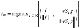
to provide the desired shift. Assuming the inner product space examined is L 2(R (similar results hold for L 2(R[a,b)), l 2(Z), and l 2(Z[a,b))), this produces
(15.17)

Since f and w are time limited to the same interval
(15.18)
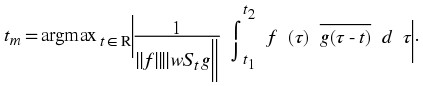
Making the subsitution  ,
,
(15.19)

Noting that this expression contains a convolution operation
(15.20)

where h is the conjugate of the time reversed version of g defined by 
In the special case in which the target signal f is not time limited, w has unit value on the entire real line. Thus, the norm can be evaluated as ||w
S
t
g|| = ||S
t
g|| = ||g|| = ||h||. Therefore, the function reduces to  where
where  The function
 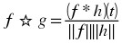 is known as the normalized cross-correlation of f and g .
Hence, this matched filter scheme can be implemented as a convolution. Therefore, it may be expedient to implement it in the frequency domain. Similar results hold for the L 2(R[a,b)), l 2(Z), and l 2(Z[a,b]) spaces. It is especially useful to implement the l 2(Z[a,b]) cases in the frequency domain as the power of the Fast Fourier Transform algorithm can be leveraged to quickly perform the computations in a computer program. In the L 2(R[a,b)) and l 2(Z[a,b]) cases, care must be taken to zero pad the signal if wrap-around effects are not desired. Similar results also hold for spaces on higher dimensional intervals with the same inner products.
Of course, there is not necessarily exactly one instance of a target signal in a given signal. There could be one instance, more than one instance, or no instance of a target signal. Therefore, it is often more practical to identify all shifts corresponding to local maxima that are above a certain threshold.
Example 15.7.
The signal in Figure 15.12 contains an instance of the template signal seen in Figure 15.11 beginning at time t = s 1 as shown by the plot in Figure 15.13. Therefore,
(15.21)
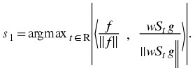
Figure 15.11. Pattern Signal
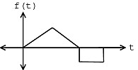
This function shows tha pattern we are looking for in the signal below, which occurs at time t = s 1 .
Figure 15.12. Longer Signal

This signal contains an instance of the above signal starting at time t = s 1 .
Figure 15.13. Absolute Value of Output
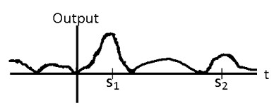
This signal shows a sketch of the absolute value of the matched filter output for the interval shown. Note that this was just an "eyeball approximation" sketch. Observe the pronounced peak at time t = s 1 .
Cauchy-Schwarz Inequality Video Lecture
Figure 15.14. Proof of the Cauchy-Schwarz Inequality
(This media type is not supported in this reader. Click to open media in browser.)
Video lecture on the proof of the Cauchy-Schwarz inequality from Khan Academy. Only part of the theorem is proven.
Cauchy-Schwarz Inequality Summary
As can be seen, the Cauchy-Schwarz inequality is a property of inner product spaces over real or complex fields that is of particular importance to the study of signals. Specifically, the implication that the absolute value of an inner product is maximized over normal vectors when the two arguments are linearly dependent is key to the justification of the matched filter detector. Thus, it enables the use of matched filters for such pattern matching applications as image detection, communications demodulation, and radar signal analysis.
15.7. Common Hilbert Spaces*
Common Hilbert Spaces
Below we will look at the four most common Hilbert spaces that you will have to deal with when discussing and manipulating signals and systems.
ℝn (reals scalars) and ℂn (complex scalars), also called ℓ 2([0, n − 1])
 is a list of numbers (finite sequence). The inner product for our two spaces are as follows:
Standard inner product ℝn :
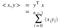
Standard inner product ℂn :
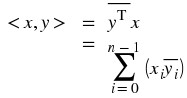
Model for: Discrete time signals on the interval [0, n − 1] or periodic (with period n ) discrete time signals. 
Figure 15.15.
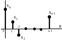
 is a finite energy function on [a, b]
(15.22)
Inner Product
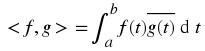
Model for: continuous time signals on the interval [a, b] or periodic (with period T = b − a ) continuous time signals
x ∈ ℓ 2(ℤ) is an infinite sequence of numbers that's square-summable
(15.23)
Inner product

Model for: discrete time, non-periodic signals
f ∈ L 2(ℝ) is a finite energy function on all of ℝ.
(15.24)
Inner product
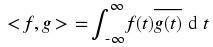
Model for: continuous time, non-periodic signals
Associated Fourier Analysis
Each of these 4 Hilbert spaces has a type of Fourier analysis associated with it.
L 2([a, b]) → Fourier series
 → Discrete Fourier Transform
 L 2(ℝ) → Fourier Transform
ℓ 2(ℤ) → Discrete Time Fourier Transform
But all 4 of these are based on the same principles (Hilbert space).
Important note
Not all normed spaces are Hilbert spaces
For example:  , ∥ f ∥ 1 = ∫|f(t)|dt . Try as you might, you can't find an inner product that induces this norm, i.e. a < ·,· > such that
 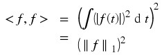 In fact, of all the L
p
(ℝ) spaces, L
2(ℝ) is the only one that is a Hilbert space.
In fact, of all the L
p
(ℝ) spaces, L
2(ℝ) is the only one that is a Hilbert space.
Figure 15.16.
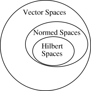
Hilbert spaces are by far the nicest. If you use or study orthonormal basis expansion then you will start to see why this is true.
15.8. Types of Bases*
Normalized Basis
Definition: Normalized Basis
a basis {b i } where each b i has unit norm ∥ b i ∥ = 1 , i ∈ ℤ
Note
The concept of basis applies to all vector spaces. The concept of normalized basis applies only to normed spaces.
You can always normalize a basis: just multiply each basis vector by a constant, such as 
Example 15.8.
We are given the following basis:Normalized with ℓ 2 norm:

Normalized with ℓ 1 norm:


Orthogonal Basis
Definition: Orthogonal Basis
a basis {b i } in which the elements are mutually orthogonal < b i ,b j > = 0 , i ≠ j
Note
The concept of orthogonal basis applies only to Hilbert Spaces.
Example 15.9.
Standard basis for ℝ 2 , also referred to as ℓ 2([0, 1]) :

Example 15.10.
Now we have the following basis and relationship:

Orthonormal Basis
Pulling the previous two sections (definitions) together, we arrive at the most important and useful basis type:
Definition: Orthonormal Basis
a basis that is both normalized and orthogonal ∥ b i ∥ = 1 , i ∈ ℤ < b i ,b j > , i ≠ j
Notation
We can shorten these two statements into one: < b i ,b j > = δ ij whereWhere δ ij is referred to as the Kronecker delta function and is also often written as δ[i − j] .
Example 15.11. Orthonormal Basis Example #1
Example 15.12. Orthonormal Basis Example #2
Example 15.13. Orthonormal Basis Example #3
Beauty of Orthonormal Bases
Orthonormal bases are very easy to deal with! If {b
i
} is an orthonormal basis, we can write for any x  It is easy to find the α
i
:
It is easy to find the α
i
:  where in the above equation we can use our knowledge of the delta function to reduce this equation:
  < x,b
i
> = α
i
Therefore, we can conclude the following important equation for x :
< x,b
i
> = α
i
Therefore, we can conclude the following important equation for x :  The α
i
's are easy to compute (no interaction between the b
i
's)
The α
i
's are easy to compute (no interaction between the b
i
's)
Example 15.14.
Given the following basis:represent

Example 15.15. Slightly Modified Fourier Series
We are given the basison
where
.
Where we can calculate the above inner product in L 2 as
Orthonormal Basis Expansions in a Hilbert Space
Let {b
i
} be an orthonormal basis for a Hilbert space H . Then, for any x ∈ H we can write  where α
i
= < x,b
i
> .
where α
i
= < x,b
i
> .
"Analysis": decomposing x in term of the b i α i = < x,b i >
"Synthesis": building x up out of a weighted combination of the b i

15.9. Orthonormal Basis Expansions*
Main Idea
When working with signals many times it is helpful to break up a signal into smaller, more manageable parts. Hopefully by now you have been exposed to the concept of eigenvectors and there use in decomposing a signal into one of its possible basis. By doing this we are able to simplify our calculations of signals and systems through eigenfunctions of LTI systems.
Now we would like to look at an alternative way to represent signals, through the use of orthonormal basis. We can think of orthonormal basis as a set of building blocks we use to construct functions. We will build up the signal/vector as a weighted sum of basis elements.
Example 15.16.
The complex sinusoidsfor all – ∞ < n < ∞ form an orthonormal basis for
.
In our Fourier series equation,, the
are just another representation of f(t) .
Note
For signals/vectors in a Hilbert Space, the expansion coefficients are easy to find.
Alternate Representation
Recall our definition of a basis: A set of vectors {b i } in a vector space S is a basis if
The b i are linearly independent.
The b i span S . That is, we can find {α i } , where α i ∈ ℂ (scalars) such that
 where x is a vector in S , α is a scalar in ℂ, and b is a vector in S .
Condition 2 in the above definition says we can decompose any vector in terms of the {b i } . Condition 1 ensures that the decomposition is unique (think about this at home).
Note
The {α i } provide an alternate representation of x .
Example 15.17.
Let us look at simple example in ℝ 2 , where we have the following vector:Standard Basis:

Alternate Basis:

In general, given a basis  and a vector x ∈ ℝ
2 , how do we find the α
0 and α
1 such that
and a vector x ∈ ℝ
2 , how do we find the α
0 and α
1 such that 
Finding the Coefficients
Now let us address the question posed above about finding α
i
's in general for ℝ
2 . We start by rewriting Equation so that we can stack our  's as columns in a 2×2 matrix.
Example 15.18.
Here is a simple example, which shows a little more detail about the above equations.
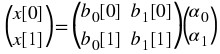
Simplifying our Equation
To make notation simpler, we define the following two items from the above equations:
Basis Matrix:

Coefficient Vector:

This gives us the following, concise equation: x = Bα which is equivalent to  .
.
Example 15.19.
Given a standard basis,, then we have the following basis matrix:

To get the α i 's, we solve for the coefficient vector in Equation α = B -1 x Where B -1 is the inverse matrix of B .
Examples
Example 15.20.
Let us look at the standard basis first and try to calculate α from it.Where I is the identity matrix. In order to solve for α let us find the inverse of B first (which is obviously very trivial in this case):
Therefore we get, α = B -1 x = x
Example 15.21.
Let us look at a ever-so-slightly more complicated basis ofThen our basis matrix and inverse basis matrix becomes:

and for this example it is given that
Now we solve for α
and we get
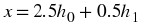
Exercise 15.9.1. (Go to Solution)
Now we are given the following basis matrix and x : 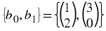
 For this problem, make a sketch of the bases and then represent x in terms of
  and
and  .
.
Note
A change of basis simply looks at x from a "different perspective." B -1 transforms x from the standard basis to our new basis,. Notice that this is a totally mechanical procedure.
Extending the Dimension and Space
We can also extend all these ideas past just ℝ
2 and look at them in ℝ
n
and ℂ
n
. This procedure extends naturally to higher (> 2) dimensions. Given a basis  for ℝ
n
, we want to find {α
0, α
1, …, α
n − 1 } such that
for ℝ
n
, we want to find {α
0, α
1, …, α
n − 1 } such that  Again, we will set up a basis matrix
  where the columns equal the basis vectors and it will always be an n×n matrix (although the above matrix does not appear to be square since we left terms in vector notation). We can then proceed to rewrite Equation
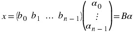 and α = B
-1
x
and α = B
-1
x
Solutions to Exercises
Solution to Exercise 15.9.1. (Return to Exercise)
In order to represent x in terms of  and
and  we will follow the same steps we used in the above example.
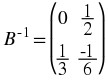
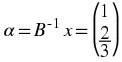 And now we can write x in terms of
  and
and  .
. 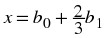 And we can easily substitute in our known values of
  and
and  to verify our results.
15.10. Function Space*
We can also find basis vectors for vector spaces other than ℝn .
Let P n be the vector space of n-th order polynomials on (-1, 1) with real coefficients (verify P 2 is a v.s. at home).
Example 15.22.
P 2 = {all quadratic polynomials}. Let b 0(t) = 1 , b 1(t) = t , b 2(t) = t 2 .
{b 0(t), b 1(t), b 2(t)} span P 2 , i.e. you can write any f(t) ∈ P 2 as f(t) = α 0 b 0(t) + α 1 b 1(t) + α 2 b 2(t) for some α i ∈ ℝ .
Note
P 2 is 3 dimensional.
f(t) = t 2 − 3t − 4
Alternate basiswrite f(t) in terms of this new basis d 0(t) = b 0(t) , d 1(t) = b 1(t) ,
. f(t) = t 2 − 3t − 4 = 4b 0(t) − 3b 1(t) + b 2(t)

so
β 1 = -3
then we get
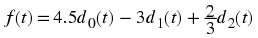
Example 15.23.
is a basis for L 2([0, T]) ,
,
.
We calculate the expansion coefficients with
(15.25)
"change of basis" formula
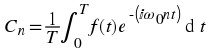
Note
There are an infinite number of elements in the basis set, that means L 2([0, T]) is infinite dimensional (scary!).
Infinite-dimensional spaces are hard to visualize. We can get a handle on the intuition by recognizing they share many of the same mathematical properties with finite dimensional spaces. Many concepts apply to both (like "basis expansion"). Some don't (change of basis isn't a nice matrix formula).
15.11. Haar Wavelet Basis*
Introduction
Fourier series is a useful orthonormal representation on L 2([0, T]) especiallly for inputs into LTI systems. However, it is ill suited for some applications, i.e. image processing (recall Gibb's phenomena).
Wavelets, discovered in the last 15 years, are another kind of basis for L 2([0, T]) and have many nice properties.
Basis Comparisons
Fourier series - c n give frequency information. Basis functions last the entire interval.
Figure 15.17.
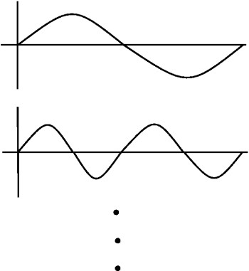
Fourier basis functions
Wavelets - basis functions give frequency info but are local in time.
Figure 15.18.
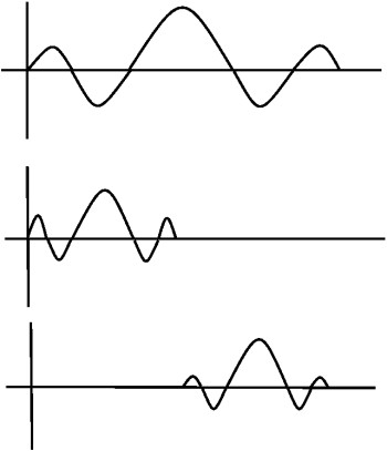
Wavelet basis functions
In Fourier basis, the basis functions are harmonic multiples of ⅇ ⅈ ω 0 t
Figure 15.19.
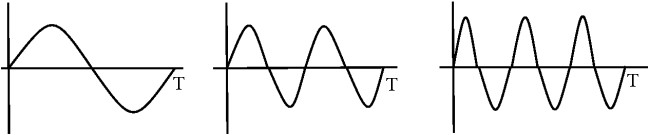
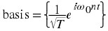
In Haar wavelet basis, the basis functions are scaled and translated versions of a "mother wavelet" ψ(t) .
Figure 15.20.
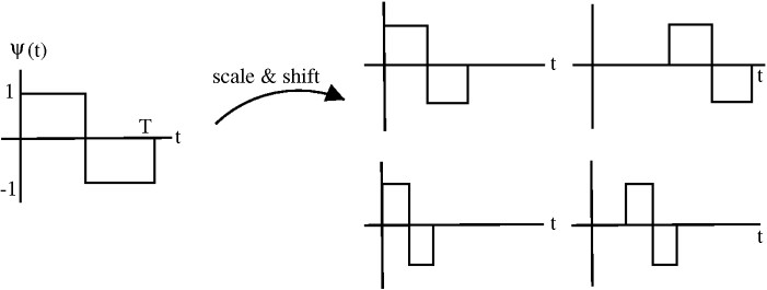
Basis functions {ψ j , k (t)} are indexed by a scale j and a shift k.
Let φ(t) = 1 , 0 ≤ t < T Then 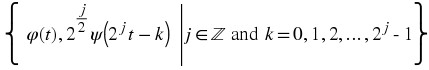
Figure 15.21.
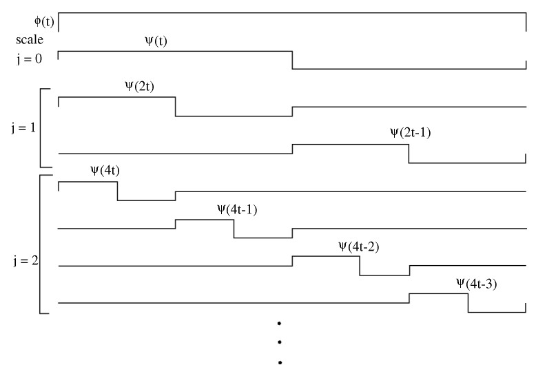
(15.26)
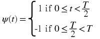
Figure 15.22.
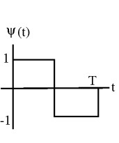
Let 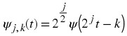
Figure 15.23.
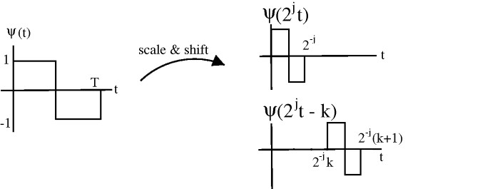
Larger j → "skinnier" basis function, j = {0, 1, 2, …} , 2j shifts at each scale: k = 0 , 1 , … , 2j – 1
Check: each ψ j , k (t) has unit energy
Figure 15.24.
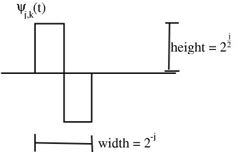
(15.27)
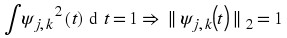
Any two basis functions are orthogonal.
Figure 15.25.
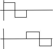
(a) Same scale

(b) Different scale
Integral of product = 0
Also, {ψ j , k , φ} span L 2([0, T])
Haar Wavelet Transform
Using what we know about Hilbert spaces: For any f(t) ∈ L 2([0, T]) , we can write
(15.28)
Synthesis
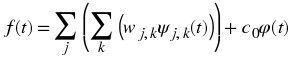
(15.29)
Analysis
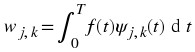
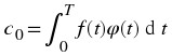
Note
the w j , k are real
The Haar transform is super useful especially in image compression
Haar Wavelet Demonstration
Figure 15.26.
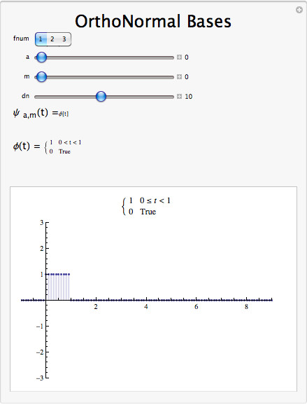
Interact (when online) with a Mathematica CDF demonstrating the Haar Wavelet as an Orthonormal Basis.
15.12. Orthonormal Bases in Real and Complex Spaces*
Notation
Transpose operator A
T flips the matrix across it's diagonal. 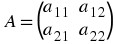
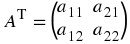 Column
i of A is row
i of A
T
Column
i of A is row
i of A
T
Recall, inner product


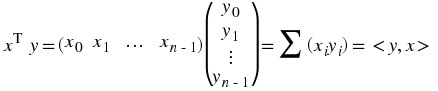 on ℝn
on ℝn
Hermitian transpose A
H , transpose and conjugate 
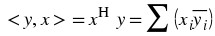 on ℂn
on ℂn
Now, let 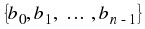 be an orthonormal basis for ℂn


Basis matrix: 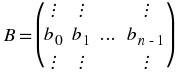 Now,
Now, 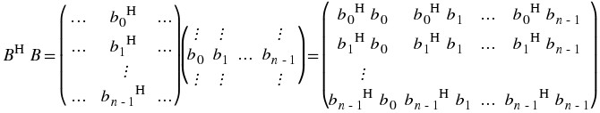
For orthonormal basis with basis matrix B B H = B -1 ( B T = B -1 in ℝn ) B H is easy to calculate while B -1 is hard to calculate.
So, to find {α 0, α 1, …, α n – 1 } such that x = ∑(α i b i ) Calculate α = B -1 x ⇒ α = B H x Using an orthonormal basis we rid ourselves of the inverse operation.
15.13. Plancharel and Parseval's Theorems*
Parseval's Theorem
Continuous Time Fourier Series preserves signal energy
i.e.:
(15.30)
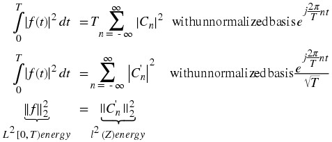
Prove: Plancherel theorem
(15.31)
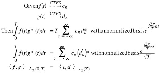
Periodic Signals Power
(15.32)
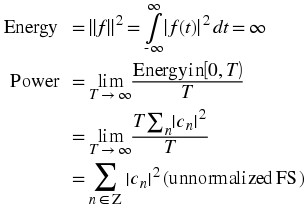
Example 15.24. Fourier Series of square pulse III -- Compute the Energy
Figure 15.27.
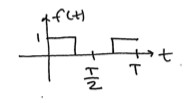
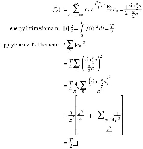
Plancharel Theorem
Theorem 15.1. Plancharel Theorem
The inner product of two vectors/signals is the same as the ℓ 2 inner product of their expansion coefficients.
Let {b
i
} be an orthonormal basis for a Hilbert Space H . x ∈ H , y ∈ H x = ∑(α
i
b
i
) y = ∑(β
i
b
i
) then 
Example 15.25.
Applying the Fourier Series, we can go from f(t) to {c n } and g(t) to {d n }inner product in time-domain = inner product of Fourier coefficients.
Proof
x = ∑(α
i
b
i
) y = ∑(β
j
b
j
)  by using inner product rules
Note
< b i ,b j > = 0 when i ≠ j and < b i ,b j > = 1 when i = j
If Hilbert space H has a ONB, then inner products are equivalent to inner products in ℓ 2 .
All H with ONB are somehow equivalent to ℓ 2 .
Point of interest
square-summable sequences are important
Plancharels Theorem Demonstration
Figure 15.28.
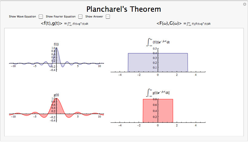
Interact (when online) with a Mathematica CDF demonstrating Plancharels Theorem visually. To Download, right-click and save target as .cdf.
Parseval's Theorem: a different approach
Theorem 15.2. Parseval's Theorem
Energy of a signal = sum of squares of its expansion coefficients
Let x ∈ H , {b i } ONB
x = ∑(α i b i ) Then ( ∥ x ∥ H )2 = ∑((|α i |)2)
Proof
Directly from Plancharel 
Example 15.26.
Fourier Series
15.14. Approximation and Projections in Hilbert Space*
Introduction
Given a line 'l' and a point 'p' in the plane, what's the closest point 'm' to 'p' on 'l'?
Figure 15.29.

Figure of point 'p' and line 'l' mentioned above.
Same problem: Let x and v be vectors in ℝ2 . Say ∥ v ∥ = 1 . For what value of α is  minimized? (what point in span{v} best approximates
x ?)
minimized? (what point in span{v} best approximates
x ?)
Figure 15.30.
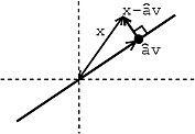
The condition is that  and αv are orthogonal.
Calculating α
How to calculate  ?
?
We know that (  ) is perpendicular to every vector in span{v}, so
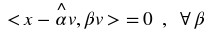
 because < v,v > = 1 , so
  Closest vector in span{v} = < x,v > v , where < x,v > v is the projection of x onto v .
We can do the same thing in higher dimensions.
Exercise 15.14.1. (Go to Solution)
Let V⊂H be a subspace of a Hilbert space H. Let x ∈ H be given. Find the y ∈ V that best approximates x . i.e., ∥ x − y ∥ is minimized.
Example 15.27.
x ∈ ℝ3 ,,
. So,

Example 15.28.
V = {space of periodic signals with frequency no greater than 3w 0 }. Given periodic f(t), what is the signal in V that best approximates f?
{
 , k = -3, -2, ..., 2, 3} is an ONB for V
  is the closest signal in V to f(t) ⇒ reconstruct f(t) using only 7 terms of its Fourier series.
Example 15.29.
Let V = {functions piecewise constant between the integers}
ONB for V.
where {b i } is an ONB.
Best piecewise constant approximation?
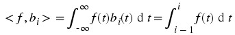
Example 15.30.
This demonstration explores approximation using a Fourier basis and a Haar Wavelet basis.See here for instructions on how to use the demo.
(This media type is not supported in this reader. Click to open media in browser.)
Solutions to Exercises
Solution to Exercise 15.14.1. (Return to Exercise)
Find an orthonormal basis {b 1, …, b k } for V
Project x onto V using
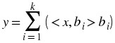 then y is the closest point in V to x and (x-y) ⊥ V ( < x − y,v > = 0 , ∀v ∈ V
Chapter 16. Appendix C: Analysis Topics Overview
16.1. Introduction to Metric Spaces*
Introduction
In may courses, concepts such as continuity and convergence are invoked without much discussion of their formal definitions, instead relying on the reader's intuitive understanding of these matters. However, for purposes of proofs, including some in the main body of material for this course, a greater rigor is required. This module will discuss metric spaces, a mathematical construct that provide a framework for the study continuity, convergence, and other related ideas in their most concrete but still formal senses. This is accomplished by formalizing a notion of the distance between two elements in a set. The intent in this and subsequent modules in this chapter is not to give a complete overview of the basic topics of analysis but to give a short introduction to those most important to discussion of signal processing in this course.
Metric Spaces
A Notion of Distance
In many situations in signal processing it is often useful to have a concept of distance between the points in a set. This notion is mathematically formalized through the idea of a metric space. A metric space (M,d) is a set M together with a function d : M × M → R that assigns distances between pairs of elements in M while satisfying three conditions. First, for every x,y ∈ M , d(x,y) ≥ 0 with d(x,y) = 0 if and only if x = y . Second, for every x,y ∈ M , d(x,y) = d(y,x) symmetrically. Third, for every x,y,z ∈ M , d(x,y) + d(x,z) ≥ d(y,z), which is known as the triangle inequality.
There are, of course, several different possible choices of definitions for distances in a given set. Our typical intuitive understanding of distance in Rn fits within this framework as the standard Euclidean metric
(16.1)d ( x , y ) = | | x – y | | 2
as does the taxicab or Manhatten metric
(16.2)d ( x , y ) = | | x – y | | 1
that sums individual components of vectors, representing, for example, distances traveled walking around city blocks. Another simple yet more exotic example is provided by the discrete metric on any set defined by
(16.3)
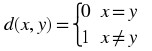
in which all pairs of distinct points are equidistant from eachother but every point is distance zero from itself. One can check that these satisfy the conditions for metric spaces.
Relationship with Norms
It is not surprising that norms, which provide a notion of size, and metrics, which provide a notion of distance, would have a close relationship. Intuitively, one way of defining the distance between two points in a metric space could be the size of their difference. In other words given a vector space V over the field F with norm || · ||, we might ask if the function
(16.4)d ( x , y ) = | | x – y | |
for every x,y ∈ V satisfies the conditions for (V,d) to be a metric space.
Let V be a vector space over the field F with norm || · ||, and let d(x,y) = ||x – y||. Recall that since || · || is a norm, ||x|| = 0 if and only if x = 0 and ||a x|| = |a|||x|| for all a ∈ F and x ∈ V . Hence ||x – y|| ≥ 0 for all x,y ∈ V and ||x – y|| = 0 if and only if x = y . Since y – x = – (x – y) and || – (x – y)|| = ||x – y|| it follows that ||x – y|| = ||y – x|| for all x,y ∈ V . Finally, ||x|| + ||y|| ≥ ||x + y|| by the properties of norms, so ||x – y|| + ||x – z|| ≥ ||y – z|| for all x,y,z ∈ V . Thus, (V,d) does indeed satisfy the conditions to be a metric space and is discussed as the metric space induced by the norm || · ||.
Metric Spaces Summary
Metric spaces provide a notion of distance and a framework with which to formally study mathematical concepts such as continuity and convergence, and other related ideas. Many metrics can be chosen for a given set, and our most common notions of distance satisfy the conditions to be a metric. Any norm on a vector space induces a metric on that vector space and it is in these types of metric spaces that we are often most interested for study of signals and systems.
16.2. Convergence of Sequences*
Introduction
Insert paragraph text here.
Sequences
Definition: sequence
A sequence is a function g n defined on the positive integers 'n '. We often denote a sequence by
Example .
A real number sequence:
Example .
A vector sequence: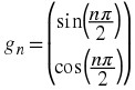
Example .
A function sequence: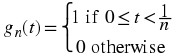
Note
A function can be thought of as an infinite dimensional vector where for each value of 't ' we have one dimension
Convergence of Real Sequences
Definition: limit
A sequenceconverges to a limit g ∈ ℝ if for every ε > 0 there is an integer N such that |g i − g| < ε , i ≥ N We usually denote a limit by writing
or g i → g
The above definition means that no matter how small we make ε , except for a finite number of g i 's, all points of the sequence are within distance ε of g .
Example 16.4.
We are given the following convergent sequence:Intuitively we can assume the following limit:
Let us prove this rigorously. Say that we are given a real number ε > 0 . Let us choose
, where ⌈x⌉ denotes the smallest integer larger than x . Then for n ≥ N we have
Thus,

Example 16.5.
Now let us look at the following non-convergent sequenceThis sequence oscillates between 1 and -1, so it will therefore never converge.
16.3. Convergence of Sequences of Vectors*
Convergence of Vectors
We now discuss pointwise and norm convergence of vectors. Other types of convergence also exist, and one in particular, uniform convergence, can also be studied. For this discussion , we will assume that the vectors belong to a normed vector space.
Pointwise Convergence
A sequence
 converges pointwise to the limit g if each element of
  converges to the corresponding element in g . Below are few examples to try and help illustrate this idea.
Example 16.6.
First we find the following limits for our two g n 's:
Therefore we have the following,
pointwise, where
.
Example 16.7.
As done above, we first want to examine the limit
where t 0 ∈ ℝ . Thus
pointwise where g(t) = 0 for all t ∈ ℝ .
Norm Convergence
The sequence
 converges to g in norm if
  . Here ∥ ˙ ∥ is the norm of the corresponding vector space of
  's. Intuitively this means the distance between vectors
  and g decreases to 0.
Example 16.8.
Let

Thus
Therefore,
in norm.
Example 16.9.
Let g(t) = 0 for all t .
Thus
Therefore, g n (t) → g(t) in norm.
Pointwise vs. Norm Convergence
Theorem 16.1.
For ℝm , pointwise and norm convergence are equivalent.
Proof: Pointwise ⇒ Norm
g
n
[i] → g[i] Assuming the above, then  Thus,
Thus, 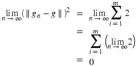
Proof: Norm ⇒ Pointwise

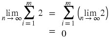 Since each term is greater than or equal zero, all 'm ' terms must be zero. Thus,
  forall i . Therefore,
Note
In infinite dimensional spaces the above theorem is no longer true. We prove this with counter examples shown below.
Counter Examples
Example 16.10. Pointwise ⇏ Norm
We are given the following function:Then
This means that, g n (t) → g(t) where for all t g(t) = 0 .
Now,Since the function norms blow up, they cannot converge to any function with finite norm.
Example 16.11. Norm ⇏ Pointwise
We are given the following function: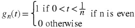
Then,
where g(t) = 0 for all t . Therefore, g n → g in norm However, at t = 0 , g n (t) oscillates between -1 and 1, and so it does not converge. Thus, g n (t) does not converge pointwise.
16.4. Uniform Convergence of Function Sequences*
Uniform Convergence of Function Sequences
For this discussion, we will only consider functions with g n where ℝ → ℝ
Definition: Uniform Convergence
The sequenceconverges uniformly to function g if for every ε > 0 there is an integer N such that n ≥ N implies |g n (t) − g(t)| ≤ ε for all t ∈ ℝ .
Obviously every uniformly convergent sequence is pointwise convergent. The difference between pointwise and uniform convergence is this: If {g n } converges pointwise to g , then for every ε > 0 and for every t ∈ ℝ there is an integer N depending on ε and t such that Equation holds if n ≥ N . If {g n } converges uniformly to g , it is possible for each ε > 0 to find one integer N that will do for all t ∈ ℝ .
Example 16.12.
Let ε > 0 be given. Then choose
. Obviously, |g n (t) − 0| ≤ ε , n ≥ N for all t . Thus, g n (t) converges uniformly to 0.
Example 16.13.
Obviously for any ε > 0 we cannot find a single function g n (t) for which Equation holds with g(t) = 0 for all t . Thus g n is not uniformly convergent. However we do have: g n (t) → g(t) pointwise
Conclusion
Uniform convergence always implies pointwise convergence, but pointwise convergence does not guarantee uniform convergence.
Chapter 17. Appendix D: Viewing Interactive Content
17.1. Viewing Embedded LabVIEW Content in Connexions*
Introduction
In order to view LabVIEW content embedded in Connexions modules, you must install and enable the LabVIEW 8.0 and 8.5 Local VI Execution Browser Plug-in for Windows. Step-by-step installation instructions are given below. Once installation is complete, the placeholder box at the bottom of this module should display a demo LabVIEW virtual instrument (VI).
Installing the LabVIEW Run-time Engine on Microsoft Windows
Download and install the LabVIEW 8.0 Runtime Engine found at: http://zone.ni.com/devzone/cda/tut/p/id/4346.
Download and install the LabVIEW 8.5 Runtime Engine found at: http://zone.ni.com/devzone/cda/tut/p/id/6633.
Dowload the LVBrowserPlugin.ini file from http://zone.ni.com/devzone/cda/tut/p/id/8288, and place it in the My Documents\LabVIEW Data folder. (You may have to create this folder if it doesn't already exist.)
Restart your computer to complete the installation.
The placeholder box at the bottom of this module should now display a demo LabVIEW virtual instrument (VI).
Example Virtual Instrument
Figure 17.1.
(This media type is not supported in this reader. Click to open media in browser.)
Digital filter design LabVIEW virtual instrument from http://cnx.org/content/m13115/latest/.
17.2. Getting Started With Mathematica*
What is Mathematica?
Mathematica is a computational software program used in technical fields. It is developed by Wolfram Research. Mathematica makes it easy to visualize data and create GUIs in only a few lines of code.
How can I run, create, and find Mathematica files?
Run
The free CDF Player is available for running non-commercial Mathematica programs. The option exists of downloading source files and running on your computer, but the CDF-player comes with a plug-in for viewing dynamic content online on your web browser!
Create
Mathematica 8 is available for purchase from Wolfram. Many universities (including Rice) and companies already have a Mathematica license. Wolfram has a free, save-disabled 15-day trial version of Mathematica.
Find
Wolfram has thousands of Mathematica programs (including source code) available at the Wolfram Demonstrations Project. Anyone can create and submit a Demonstration. Also, many other websites (including Connexions) have a lot of Mathematica content.
What do I need to run interactive content?
Mathematica 8 is supported on Linux, Microsoft Windows, Mac OS X, and Solaris. Mathematica's free CDF-player is available for Windows and Mac OS X, and is in development for Linux; the CDF-Player plugin is available for IE, Firefox, Chrome, Safari, and Opera.
How can I upload a Mathematica file to a Connexions module?
Go to the Files tab at the top of the module and upload your .cdf file, along with an (optional) screenshot of the file in use. In order to generate a clean bracket-less screenshot, you should do the following:
Open your .cdf in Mathematica and left click on the bracket surrounding the manipulate command.
Click on Cell->Convert To->Bitmap.
Then click on File->Save Selection As, and save the image file in your desired image format.
Embed the files into the module in any way you like. Some tags you may find helpful include image, figure, download, and link (if linking to an .cdf file on another website). The best method is to create an interactive figure, and include a fallback png image of the cdf file should the CDF image not render properly. See the interactive demo/image below.
Convolution Demo
<figure id="demoonline">
<media id="CNXdemoonline" alt="timeshiftDemo">
<image mime-type="image/png" src="Convolutiondisplay-4.cdf" thumbnail="Convolution4.0Display.png" width="600"/>
<object width="500" height="500" src="Convolutiondisplay-4.cdf" mime-type="application/vnd.wolfram.cdf" for="webview2.0"/>
<image mime-type="application/postscript" for="pdf" src="Convolution4.0Display.png" width="400"/>
</media>
<caption>Interact (when online) with a Mathematica CDF demonstrating Convolution. To Download, right-click and save target as .cdf.%lt;/caption>
</figure>
Figure 17.2.
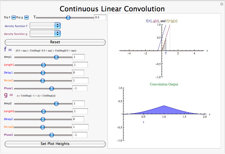
Interact (when online) with a Mathematica CDF demonstrating Convolution. To Download, right-click and save target as .cdf.
Alternatively, this is how it looks when you use a thumbnail link to a live online demo.
Figure 17.3.

Click on the above thumbnail image (when online) to view an interactive Mathematica Player demonstrating Convolution.
How can I learn Mathematica?
Open Mathematica and go to the Getting Started section of the "Welcome to Mathematica" screen, or check out Help: Documentation Center.
The Mathematica Learning Center has lots of screencasts, how-tos, and tutorials.
When troubleshooting, the error messages are often unhelpful, so it's best to evaluate often so the problem can be easily located. Search engines like Google are useful when you're looking for an explanation of specific error messages.
Appendix A. Attributions
| Collection: Signals and Systems |
| Edited by: Richard Baraniuk |
| Edited by: Catherine Elder, Chinwei Hu, Stephen Kruzick, Dante Soares, Catherine Elder, Chinwei Hu, Stephen Kruzick, and Dante Soares |
| URL: http://cnx.org/content/col10064/1.14/ |
| Copyright: Richard Baraniuk |
| License: http://creativecommons.org/licenses/by/3.0/ |
| Module: Signal Classifications and Properties |
| By: Melissa Selik, Richard Baraniuk, and Michael Haag |
| URL: http://cnx.org/content/m10057/2.21/ |
| Copyright: Melissa Selik, Richard Baraniuk, and Michael Haag |
| License: http://creativecommons.org/licenses/by/1.0 |
| Module: Signal Size and Norms |
| By: Richard Baraniuk and Stephen Kruzick |
| URL: http://cnx.org/content/m12363/1.4/ |
| Copyright: Richard Baraniuk and Stephen Kruzick |
| License: http://creativecommons.org/licenses/by/1.0 |
| Module: Signal Operations |
| By: Richard Baraniuk |
| URL: http://cnx.org/content/m10125/2.17/ |
| Copyright: Richard Baraniuk and Adam Blair |
| License: http://creativecommons.org/licenses/by/3.0/ |
| Module: Common Continuous Time Signals |
| By: Melissa Selik and Richard Baraniuk |
| URL: http://cnx.org/content/m10058/2.15/ |
| Copyright: Melissa Selik and Richard Baraniuk |
| License: http://creativecommons.org/licenses/by/1.0 |
| Module: Common Discrete Time Signals |
| By: Stephen Kruzick |
| URL: http://cnx.org/content/m34575/1.2/ |
| Copyright: Stephen Kruzick |
| License: http://creativecommons.org/licenses/by/3.0/ |
| Based on: Discrete-Time Signals <http://cnx.org/content/m0009/2.24> by Don Johnson. |
| Module: Continuous Time Impulse Function |
| By: Melissa Selik and Richard Baraniuk |
| URL: http://cnx.org/content/m10059/2.26/ |
| Copyright: Melissa Selik, Richard Baraniuk, and Adam Blair |
| License: http://creativecommons.org/licenses/by/3.0/ |
| Module: Discrete Time Impulse Function |
| By: Dan Calderon |
| URL: http://cnx.org/content/m34566/1.6/ |
| Copyright: Dan Calderon |
| License: http://creativecommons.org/licenses/by/3.0/ |
| Module: Continuous Time Complex Exponential |
| By: Richard Baraniuk and Stephen Kruzick |
| URL: http://cnx.org/content/m10060/2.24/ |
| Copyright: Richard Baraniuk, Stephen Kruzick, and Adam Blair |
| License: http://creativecommons.org/licenses/by/3.0/ |
| Module: Discrete Time Complex Exponential |
| By: Dan Calderon, Richard Baraniuk, and Stephen Kruzick |
| URL: http://cnx.org/content/m34573/1.3/ |
| Copyright: Dan Calderon and Stephen Kruzick |
| License: http://creativecommons.org/licenses/by/3.0/ |
| Based on: The Complex Exponential <http://cnx.org/content/m10060/2.21> by Richard Baraniuk. |
| Module: System Classifications and Properties |
| By: Melissa Selik, Richard Baraniuk, and Stephen Kruzick |
| URL: http://cnx.org/content/m10084/2.21/ |
| Copyright: Melissa Selik, Richard Baraniuk, and Stephen Kruzick |
| License: http://creativecommons.org/licenses/by/1.0 |
| Module: Linear Time Invariant Systems |
| By: Thanos Antoulas and John Slavinsky |
| URL: http://cnx.org/content/m2102/2.24/ |
| Copyright: Thanos Antoulas and John Slavinsky |
| License: http://creativecommons.org/licenses/by/3.0/ |
| Module: Continuous Time Systems |
| By: Michael Haag, Richard Baraniuk, and Stephen Kruzick |
| URL: http://cnx.org/content/m10855/2.8/ |
| Copyright: Michael Haag, Richard Baraniuk, and Stephen Kruzick |
| License: http://creativecommons.org/licenses/by/1.0 |
| Module: Continuous Time Impulse Response |
| By: Dante Soares |
| URL: http://cnx.org/content/m34629/1.1/ |
| Copyright: Dante Soares |
| License: http://creativecommons.org/licenses/by/3.0/ |
| Module: Continuous Time Convolution |
| By: Melissa Selik, Richard Baraniuk, Stephen Kruzick, and Dan Calderon |
| URL: http://cnx.org/content/m10085/2.34/ |
| Copyright: Melissa Selik, Richard Baraniuk, Stephen Kruzick, Dan Calderon, and Adam Blair |
| License: http://creativecommons.org/licenses/by/3.0/ |
| Module: Properties of Continuous Time Convolution |
| By: Melissa Selik, Richard Baraniuk, and Stephen Kruzick |
| URL: http://cnx.org/content/m10088/2.17/ |
| Copyright: Melissa Selik, Richard Baraniuk, and Stephen Kruzick |
| License: http://creativecommons.org/licenses/by/1.0 |
| Module: Eigenfunctions of Continuous Time LTI Systems |
| By: Stephen Kruzick |
| URL: http://cnx.org/content/m34639/1.1/ |
| Copyright: Stephen Kruzick |
| License: http://creativecommons.org/licenses/by/3.0/ |
| Based on: Eigenfunctions of LTI Systems <http://cnx.org/content/m10500/2.8> by Justin Romberg. |
| Module: BIBO Stability of Continuous Time Systems |
| By: Richard Baraniuk and Stephen Kruzick |
| URL: http://cnx.org/content/m10113/2.11/ |
| Copyright: Richard Baraniuk and Stephen Kruzick |
| License: http://creativecommons.org/licenses/by/1.0 |
| Module: Linear Constant Coefficient Differential Equations |
| By: Stephen Kruzick |
| URL: http://cnx.org/content/m34501/1.4/ |
| Copyright: Stephen Kruzick |
| License: http://creativecommons.org/licenses/by/3.0/ |
| Module: Solving Linear Constant Coefficient Differential Equations |
| By: Stephen Kruzick |
| URL: http://cnx.org/content/m34506/1.4/ |
| Copyright: Stephen Kruzick |
| License: http://creativecommons.org/licenses/by/3.0/ |
| Module: Discrete Time Systems |
| By: Stephen Kruzick |
| URL: http://cnx.org/content/m34614/1.2/ |
| Copyright: Stephen Kruzick |
| License: http://creativecommons.org/licenses/by/3.0/ |
| Based on: Discrete-Time Systems in the Time-Domain <http://cnx.org/content/m10251/2.23> by Don Johnson. |
| Module: Discrete Time Impulse Response |
| By: Dante Soares |
| URL: http://cnx.org/content/m34626/1.1/ |
| Copyright: Dante Soares |
| License: http://creativecommons.org/licenses/by/3.0/ |
| Module: Discrete Time Convolution |
| By: Ricardo Radaelli-Sanchez, Richard Baraniuk, Stephen Kruzick, and Catherine Elder |
| Edited by: Catherine Elder |
| URL: http://cnx.org/content/m10087/2.27/ |
| Copyright: Ricardo Radaelli-Sanchez, Richard Baraniuk, and Stephen Kruzick |
| License: http://creativecommons.org/licenses/by/3.0/ |
| Module: Properties of Discrete Time Convolution |
| By: Stephen Kruzick |
| URL: http://cnx.org/content/m34625/1.2/ |
| Copyright: Stephen Kruzick |
| License: http://creativecommons.org/licenses/by/3.0/ |
| Module: Eigenfunctions of Discrete Time LTI Systems |
| By: Stephen Kruzick |
| URL: http://cnx.org/content/m34640/1.1/ |
| Copyright: Stephen Kruzick |
| License: http://creativecommons.org/licenses/by/3.0/ |
| Based on: Eigenfunctions of LTI Systems <http://cnx.org/content/m10500/2.8> by Justin Romberg. |
| Module: BIBO Stability of Discrete Time Systems |
| By: Stephen Kruzick |
| URL: http://cnx.org/content/m34515/1.2/ |
| Copyright: Stephen Kruzick |
| License: http://creativecommons.org/licenses/by/3.0/ |
| Based on: BIBO Stability <http://cnx.org/content/m10113/2.10> by Richard Baraniuk. |
| Module: Linear Constant Coefficient Difference Equations |
| By: Richard Baraniuk and Stephen Kruzick |
| URL: http://cnx.org/content/m12325/1.4/ |
| Copyright: Richard Baraniuk and Stephen Kruzick |
| License: http://creativecommons.org/licenses/by/1.0 |
| Module: Solving Linear Constant Coefficient Difference Equations |
| By: Richard Baraniuk and Stephen Kruzick |
| URL: http://cnx.org/content/m12326/1.5/ |
| Copyright: Richard Baraniuk and Stephen Kruzick |
| License: http://creativecommons.org/licenses/by/1.0 |
| Module: Introduction to Fourier Analysis |
| By: |
| URL: http://cnx.org/content/id386622/2.12/ |
| Module: Introduction to Fourier Analysis |
| By: Richard Baraniuk |
| URL: http://cnx.org/content/m10096/2.12/ |
| Copyright: Richard Baraniuk |
| License: http://creativecommons.org/licenses/by/1.0 |
| Module: Continuous Time Periodic Signals |
| By: Michael Haag and Justin Romberg |
| URL: http://cnx.org/content/m10744/2.13/ |
| Copyright: Michael Haag and Justin Romberg |
| License: http://creativecommons.org/licenses/by/3.0/ |
| Module: Continuous Time Fourier Series (CTFS) |
| By: Stephen Kruzick and Dan Calderon |
| URL: http://cnx.org/content/m34531/1.9/ |
| Copyright: Stephen Kruzick and Dan Calderon |
| License: http://creativecommons.org/licenses/by/3.0/ |
| Module: Common Fourier Series |
| By: Dan Calderon and Don Johnson |
| URL: http://cnx.org/content/m34770/1.7/ |
| Copyright: Dan Calderon |
| License: http://creativecommons.org/licenses/by/3.0/ |
| Based on: Fourier Series Approximation of Signals <http://cnx.org/content/m10687/2.9> by Don Johnson. |
| Module: Properties of the CTFS |
| By: Justin Romberg and Benjamin Fite |
| URL: http://cnx.org/content/m10740/2.15/ |
| Copyright: Justin Romberg and Benjamin Fite |
| License: http://creativecommons.org/licenses/by/3.0/ |
| Module: Continuous Time Circular Convolution and the CTFS |
| By: Justin Romberg |
| URL: http://cnx.org/content/m10839/2.6/ |
| Copyright: Justin Romberg and Richard Baraniuk |
| License: http://creativecommons.org/licenses/by/1.0 |
| Module: Existence and Convergence of Fourier Series |
| Used here as: Convergence of Fourier Series |
| By: Michael Haag and Justin Romberg |
| URL: http://cnx.org/content/m10745/2.5/ |
| Copyright: Michael Haag and Justin Romberg |
| License: http://creativecommons.org/licenses/by/1.0 |
| Module: Gibbs Phenomena |
| By: Ricardo Radaelli-Sanchez and Richard Baraniuk |
| URL: http://cnx.org/content/m10092/2.14/ |
| Copyright: Ricardo Radaelli-Sanchez and Richard Baraniuk |
| License: http://creativecommons.org/licenses/by/3.0/ |
| Module: Discrete Time Periodic Signals |
| By: Stephen Kruzick and Dan Calderon |
| URL: http://cnx.org/content/m34824/1.5/ |
| Copyright: Stephen Kruzick and Dan Calderon |
| License: http://creativecommons.org/licenses/by/3.0/ |
| Module: Discrete Time Fourier Series (DTFS) |
| By: Michael Haag and Justin Romberg |
| URL: http://cnx.org/content/m10784/2.14/ |
| Copyright: Michael Haag and Justin Romberg |
| License: http://creativecommons.org/licenses/by/3.0/ |
| Module: Common Discrete Fourier Series |
| By: Stephen Kruzick |
| URL: http://cnx.org/content/m34509/1.8/ |
| Copyright: Stephen Kruzick |
| License: http://creativecommons.org/licenses/by/3.0/ |
| Module: Properties of the DTFS |
| By: Stephen Kruzick |
| URL: http://cnx.org/content/m34508/1.7/ |
| Copyright: Stephen Kruzick |
| License: http://creativecommons.org/licenses/by/3.0/ |
| Module: Discrete Time Circular Convolution and the DTFS |
| By: Justin Romberg |
| URL: http://cnx.org/content/m10786/2.14/ |
| Copyright: Justin Romberg |
| License: http://creativecommons.org/licenses/by/3.0/ |
| Module: Continuous Time Aperiodic Signals |
| By: Stephen Kruzick |
| URL: http://cnx.org/content/m34848/1.5/ |
| Copyright: Stephen Kruzick |
| License: http://creativecommons.org/licenses/by/3.0/ |
| Module: Continuous Time Fourier Transform (CTFT) |
| By: Richard Baraniuk and Melissa Selik |
| URL: http://cnx.org/content/m10098/2.16/ |
| Copyright: Richard Baraniuk and Melissa Selik |
| License: http://creativecommons.org/licenses/by/3.0/ |
| Module: Common Fourier Transforms |
| By: Melissa Selik and Richard Baraniuk |
| URL: http://cnx.org/content/m10099/2.11/ |
| Copyright: Melissa Selik and Richard Baraniuk |
| License: http://creativecommons.org/licenses/by/1.0 |
| Module: Properties of the CTFT |
| By: Melissa Selik and Richard Baraniuk |
| URL: http://cnx.org/content/m10100/2.15/ |
| Copyright: Melissa Selik and Richard Baraniuk |
| License: http://creativecommons.org/licenses/by/1.0 |
| Module: Continuous Time Convolution and the CTFT |
| By: Stephen Kruzick |
| URL: http://cnx.org/content/m34849/1.4/ |
| Copyright: Stephen Kruzick |
| License: http://creativecommons.org/licenses/by/3.0/ |
| Module: Discrete Time Aperiodic Signals |
| By: Stephen Kruzick and Dan Calderon |
| URL: http://cnx.org/content/m34850/1.4/ |
| Copyright: Stephen Kruzick and Dan Calderon |
| License: http://creativecommons.org/licenses/by/3.0/ |
| Module: Discrete Time Fourier Transform (DTFT) |
| By: Richard Baraniuk |
| URL: http://cnx.org/content/m10108/2.18/ |
| Copyright: Richard Baraniuk |
| License: http://creativecommons.org/licenses/by/3.0/ |
| Module: Common Discrete Time Fourier Transforms |
| By: Stephen Kruzick |
| URL: http://cnx.org/content/m34771/1.2/ |
| Copyright: Stephen Kruzick |
| License: http://creativecommons.org/licenses/by/3.0/ |
| Module: Properties of the DTFT |
| By: Don Johnson |
| URL: http://cnx.org/content/m0506/2.7/ |
| Copyright: Don Johnson |
| License: http://creativecommons.org/licenses/by/1.0 |
| Module: Discrete Time Convolution and the DTFT |
| By: Stephen Kruzick and Dan Calderon |
| URL: http://cnx.org/content/m34851/1.4/ |
| Copyright: Stephen Kruzick and Dan Calderon |
| License: http://creativecommons.org/licenses/by/3.0/ |
| Module: Signal Sampling |
| By: Stephen Kruzick and Justin Romberg |
| URL: http://cnx.org/content/m10798/2.8/ |
| Copyright: Stephen Kruzick and Justin Romberg |
| License: http://creativecommons.org/licenses/by/1.0 |
| Module: Sampling Theorem |
| By: Justin Romberg and Stephen Kruzick |
| URL: http://cnx.org/content/m10791/2.7/ |
| Copyright: Justin Romberg and Stephen Kruzick |
| License: http://creativecommons.org/licenses/by/1.0 |
| Module: Signal Reconstruction |
| By: Stephen Kruzick and Justin Romberg |
| URL: http://cnx.org/content/m10788/2.8/ |
| Copyright: Stephen Kruzick and Justin Romberg |
| License: http://creativecommons.org/licenses/by/1.0 |
| Module: Perfect Reconstruction |
| By: Stephen Kruzick, Roy Ha, and Justin Romberg |
| URL: http://cnx.org/content/m10790/2.6/ |
| Copyright: Stephen Kruzick, Roy Ha, and Justin Romberg |
| License: http://creativecommons.org/licenses/by/1.0 |
| Module: Aliasing Phenomena |
| By: Stephen Kruzick |
| Edited by: Catherine Elder |
| URL: http://cnx.org/content/m34847/1.5/ |
| Copyright: Stephen Kruzick |
| License: http://creativecommons.org/licenses/by/3.0/ |
| Based on: Aliasing <http://cnx.org/content/m10793/2.7> by Justin Rombergand Don Johnson. |
| Module: Anti-Aliasing Filters |
| By: Justin Romberg and Stephen Kruzick |
| URL: http://cnx.org/content/m10794/2.6/ |
| Copyright: Justin Romberg and Stephen Kruzick |
| License: http://creativecommons.org/licenses/by/1.0 |
| Module: Discrete Time Processing of Continuous Time Signals |
| By: Justin Romberg and Stephen Kruzick |
| URL: http://cnx.org/content/m10797/2.11/ |
| Copyright: Justin Romberg and Stephen Kruzick |
| License: http://creativecommons.org/licenses/by/1.0 |
| Module: The Laplace Transform |
| Used here as: Laplace Transform |
| By: Richard Baraniuk and Dan Calderon |
| URL: http://cnx.org/content/m10110/2.17/ |
| Copyright: Richard Baraniuk and Dan Calderon |
| License: http://creativecommons.org/licenses/by/3.0/ |
| Module: Common Laplace Transforms |
| By: Melissa Selik and Richard Baraniuk |
| URL: http://cnx.org/content/m10111/2.13/ |
| Copyright: Melissa Selik and Richard Baraniuk |
| License: http://creativecommons.org/licenses/by/3.0/ |
| Module: Properties of the Laplace Transform |
| By: Melissa Selik and Richard Baraniuk |
| URL: http://cnx.org/content/m10117/2.11/ |
| Copyright: Melissa Selik and Richard Baraniuk |
| License: http://creativecommons.org/licenses/by/1.0 |
| Module: The Inverse Laplace Transform |
| Used here as: Inverse Laplace Transform |
| By: Dan Calderon |
| URL: http://cnx.org/content/m34857/1.1/ |
| Copyright: Dan Calderon |
| License: http://creativecommons.org/licenses/by/3.0/ |
| Based on: Inverse Z-Transform <http://cnx.org/content/m10651/2.4> by Benjamin Fite. |
| Module: Understanding Pole/Zero Plots on the S-Plane |
| Used here as: Poles and Zeros in the S-Plane |
| By: Dan Calderon |
| URL: http://cnx.org/content/m34855/1.4/ |
| Copyright: Dan Calderon |
| License: http://creativecommons.org/licenses/by/3.0/ |
| Based on: Understanding Pole/Zero Plots on the Z-Plane <http://cnx.org/content/m10556/2.8> by Michael Haag. |
| Module: Region of Convergence for the Laplace Transform |
| By: Richard Baraniuk and Dan Calderon |
| URL: http://cnx.org/content/m10114/2.11/ |
| Copyright: Richard Baraniuk and Dan Calderon |
| License: http://creativecommons.org/licenses/by/3.0/ |
| Module: Rational Functions and the Laplace Transform |
| By: Stephen Kruzick |
| URL: http://cnx.org/content/m34530/1.2/ |
| Copyright: Stephen Kruzick |
| License: http://creativecommons.org/licenses/by/3.0/ |
| Based on: Rational Functions <http://cnx.org/content/m10593/2.7> by Michael Haag. |
| Module: Differential Equations |
| By: Stephen Kruzick |
| URL: http://cnx.org/content/m34510/1.3/ |
| Copyright: Stephen Kruzick |
| License: http://creativecommons.org/licenses/by/3.0/ |
| Module: Analog Filter Design |
| Used here as: Continuous Time Filter Design |
| By: Dan Calderon and C. Burrus |
| URL: http://cnx.org/content/m34921/1.2/ |
| Copyright: Dan Calderon and C. Burrus |
| License: http://creativecommons.org/licenses/by/3.0/ |
| Based on: Filter Design using the Pole/Zero Plot of a Z-Transform <http://cnx.org/content/m10548/2.9> by Michael Haag. |
| Module: The Z Transform |
| Used here as: Z-Transform |
| By: Dan Calderon and Richard Baraniuk |
| Edited by: Chinwei Hu, Catherine Elder, Stephen Kruzick, and Dante Soares |
| URL: http://cnx.org/content/m34858/1.4/ |
| Copyright: Dan Calderon |
| License: http://creativecommons.org/licenses/by/3.0/ |
| Based on: The Laplace Transforms <http://cnx.org/content/m10110/2.13> by Richard Baraniuk. |
| Module: Common Z Transforms |
| Used here as: Common Z-Transforms |
| By: Dan Calderon |
| URL: http://cnx.org/content/m34859/1.1/ |
| Copyright: Dan Calderon |
| License: http://creativecommons.org/licenses/by/3.0/ |
| Module: Properties of the Z-Transform |
| By: Stephen Kruzick |
| URL: http://cnx.org/content/m34477/1.2/ |
| Copyright: Stephen Kruzick |
| License: http://creativecommons.org/licenses/by/3.0/ |
| Module: The Inverse Z-Transform |
| Used here as: Inverse Z-Transform |
| By: Benjamin Fite |
| URL: http://cnx.org/content/m10651/2.5/ |
| Copyright: Benjamin Fite |
| License: http://creativecommons.org/licenses/by/1.0 |
| Module: Understanding Pole/Zero Plots on the Z-Plane |
| Used here as: Poles and Zeros in the Z-Plane |
| By: Michael Haag |
| URL: http://cnx.org/content/m10556/2.12/ |
| Copyright: Michael Haag |
| License: http://creativecommons.org/licenses/by/3.0/ |
| Module: Region of Convergence for the Z-transform |
| By: Benjamin Fite and Dan Calderon |
| URL: http://cnx.org/content/m10622/2.8/ |
| Copyright: Benjamin Fite and Dan Calderon |
| License: http://creativecommons.org/licenses/by/3.0/ |
| Module: Rational Functions and the Z-Transform |
| By: Michael Haag |
| URL: http://cnx.org/content/m10593/2.8/ |
| Copyright: Michael Haag |
| License: http://creativecommons.org/licenses/by/1.0 |
| Module: Difference Equation |
| Used here as: Difference Equations |
| By: Michael Haag |
| URL: http://cnx.org/content/m10595/2.6/ |
| Copyright: Michael Haag |
| License: http://creativecommons.org/licenses/by/1.0 |
| Module: Discrete Time Filter Design |
| By: Michael Haag |
| URL: http://cnx.org/content/m10548/2.10/ |
| Copyright: Michael Haag |
| License: http://creativecommons.org/licenses/by/1.0 |
| Module: DFT: Fast Fourier Transform |
| By: Don Johnson |
| URL: http://cnx.org/content/m0504/2.8/ |
| Copyright: Don Johnson |
| License: http://creativecommons.org/licenses/by/1.0 |
| Module: The Fast Fourier Transform (FFT) |
| By: Justin Romberg |
| URL: http://cnx.org/content/m10783/2.7/ |
| Copyright: Justin Romberg |
| License: http://creativecommons.org/licenses/by/1.0 |
| Module: Deriving the Fast Fourier Transform |
| By: Don Johnson |
| URL: http://cnx.org/content/m0528/2.7/ |
| Copyright: Don Johnson |
| License: http://creativecommons.org/licenses/by/1.0 |
| Module: Matched Filter Detector |
| By: Stephen Kruzick, Dan Calderon, Catherine Elder, and Richard Baraniuk |
| URL: http://cnx.org/content/m34670/1.9/ |
| Copyright: Stephen Kruzick, Dan Calderon, Catherine Elder, and Richard Baraniuk |
| License: http://creativecommons.org/licenses/by/3.0/ |
| Based on: Cauchy-Schwarz Inequality <http://cnx.org/content/m10757/2.6> by Michael Haagand Justin Romberg. |
| Module: Linear Algebra: The Basics |
| Used here as: Basic Linear Algebra |
| By: Michael Haag and Justin Romberg |
| URL: http://cnx.org/content/m10734/2.6/ |
| Copyright: Michael Haag and Justin Romberg |
| License: http://creativecommons.org/licenses/by/1.0 |
| Module: Eigenvectors and Eigenvalues |
| By: Michael Haag and Justin Romberg |
| URL: http://cnx.org/content/m10736/2.9/ |
| Copyright: Michael Haag and Justin Romberg |
| License: http://creativecommons.org/licenses/by/1.0 |
| Module: Matrix Diagonalization |
| By: Michael Haag |
| URL: http://cnx.org/content/m10738/2.6/ |
| Copyright: Michael Haag |
| License: http://creativecommons.org/licenses/by/1.0 |
| Module: Eigen-stuff in a Nutshell |
| By: Michael Haag and Justin Romberg |
| URL: http://cnx.org/content/m10742/2.6/ |
| Copyright: Michael Haag and Justin Romberg |
| License: http://creativecommons.org/licenses/by/1.0 |
| Module: Eigenfunctions of LTI Systems |
| By: Justin Romberg |
| URL: http://cnx.org/content/m10500/2.9/ |
| Copyright: Justin Romberg |
| License: http://creativecommons.org/licenses/by/1.0 |
| Module: Fields and Complex Numbers |
| By: Stephen Kruzick |
| URL: http://cnx.org/content/m34514/1.4/ |
| Copyright: Stephen Kruzick |
| License: http://creativecommons.org/licenses/by/3.0/ |
| Based on: Complex Numbers <http://cnx.org/content/m0081/2.27> by Don Johnson. |
| Module: Vector Spaces |
| By: Michael Haag, Steven Cox, and Justin Romberg |
| URL: http://cnx.org/content/m10767/2.6/ |
| Copyright: Michael Haag, Steven Cox, and Justin Romberg |
| License: http://creativecommons.org/licenses/by/1.0 |
| Module: Norms |
| By: Michael Haag and Justin Romberg |
| URL: http://cnx.org/content/m10768/2.6/ |
| Copyright: Michael Haag and Justin Romberg |
| License: http://creativecommons.org/licenses/by/1.0 |
| Module: Inner Products |
| By: Michael Haag and Justin Romberg |
| URL: http://cnx.org/content/m10755/2.8/ |
| Copyright: Michael Haag and Justin Romberg |
| License: http://creativecommons.org/licenses/by/1.0 |
| Module: Hilbert Spaces |
| By: Justin Romberg |
| URL: http://cnx.org/content/m10840/2.6/ |
| Copyright: Justin Romberg |
| License: http://creativecommons.org/licenses/by/1.0 |
| Module: Cauchy-Schwarz Inequality |
| By: Michael Haag, Justin Romberg, Stephen Kruzick, Dan Calderon, and Catherine Elder |
| URL: http://cnx.org/content/m10757/2.7/ |
| Copyright: Michael Haag, Justin Romberg, Stephen Kruzick, Dan Calderon, and Catherine Elder |
| License: http://creativecommons.org/licenses/by/1.0 |
| Module: Common Hilbert Spaces |
| By: Roy Ha and Justin Romberg |
| URL: http://cnx.org/content/m10759/2.7/ |
| Copyright: Roy Ha and Justin Romberg |
| License: http://creativecommons.org/licenses/by/1.0 |
| Module: Types of Bases |
| By: Michael Haag and Justin Romberg |
| URL: http://cnx.org/content/m10772/2.8/ |
| Copyright: Michael Haag and Justin Romberg |
| License: http://creativecommons.org/licenses/by/3.0/ |
| Module: Orthonormal Basis Expansions |
| By: Michael Haag and Justin Romberg |
| URL: http://cnx.org/content/m10760/2.6/ |
| Copyright: Michael Haag and Justin Romberg |
| License: http://creativecommons.org/licenses/by/1.0 |
| Module: Function Space |
| By: Justin Romberg |
| URL: http://cnx.org/content/m10770/2.6/ |
| Copyright: Justin Romberg |
| License: http://creativecommons.org/licenses/by/1.0 |
| Module: Haar Wavelet Basis |
| By: Roy Ha and Justin Romberg |
| URL: http://cnx.org/content/m10764/2.9/ |
| Copyright: Roy Ha and Justin Romberg |
| License: http://creativecommons.org/licenses/by/3.0/ |
| Module: Orthonormal Bases in Real and Complex Spaces |
| By: Justin Romberg |
| URL: http://cnx.org/content/m10765/2.8/ |
| Copyright: Justin Romberg |
| License: http://creativecommons.org/licenses/by/1.0 |
| Module: Plancharel and Parseval's Theorems |
| By: Justin Romberg |
| URL: http://cnx.org/content/m10769/2.10/ |
| Copyright: Justin Romberg |
| License: http://creativecommons.org/licenses/by/3.0/ |
| Module: Approximation and Projections in Hilbert Space |
| By: Justin Romberg |
| URL: http://cnx.org/content/m10766/2.9/ |
| Copyright: Justin Romberg |
| License: http://creativecommons.org/licenses/by/1.0 |
| Module: Introduction to Metric Spaces |
| By: Stephen Kruzick |
| URL: http://cnx.org/content/m34616/1.2/ |
| Copyright: Stephen Kruzick |
| License: http://creativecommons.org/licenses/by/3.0/ |
| Module: Convergence of Sequences |
| By: Richard Baraniuk |
| URL: http://cnx.org/content/m10883/2.6/ |
| Copyright: Richard Baraniuk |
| License: http://creativecommons.org/licenses/by/1.0 |
| Module: Convergence of Vectors |
| Used here as: Convergence of Sequences of Vectors |
| By: Michael Haag |
| URL: http://cnx.org/content/m10894/2.4/ |
| Copyright: Michael Haag |
| License: http://creativecommons.org/licenses/by/1.0 |
| Module: Uniform Convergence of Function Sequences |
| By: Michael Haag and Richard Baraniuk |
| URL: http://cnx.org/content/m10895/2.7/ |
| Copyright: Michael Haag |
| License: http://creativecommons.org/licenses/by/1.0 |
| Module: Viewing Embedded LabVIEW Content in Connexions |
| By: Stephen Kruzick |
| URL: http://cnx.org/content/m34460/1.4/ |
| Copyright: Stephen Kruzick |
| License: http://creativecommons.org/licenses/by/3.0/ |
| Based on: Viewing Embedded LabVIEW Content <http://cnx.org/content/m13753/1.3> by Matthew Hutchinson. |
| Module: Getting Started With Mathematica |
| By: Catherine Elder and Dan Calderon |
| URL: http://cnx.org/content/m36728/1.12/ |
| Copyright: Catherine Elder and Dan Calderon |
| License: http://creativecommons.org/licenses/by/3.0/ |
About Connexions
Since 1999, Connexions has been pioneering a global system where anyone can create course materials and make them fully accessible and easily reusable free of charge. We are a Web-based authoring, teaching and learning environment open to anyone interested in education, including students, teachers, professors and lifelong learners. We connect ideas and facilitate educational communities. Connexions's modular, interactive courses are in use worldwide by universities, community colleges, K-12 schools, distance learners, and lifelong learners. Connexions materials are in many languages, including English, Spanish, Chinese, Japanese, Italian, Vietnamese, French, Portuguese, and Thai.


This course deals with signals, systems, and transforms, from their theoretical mathematical foundations to practical implementation in circuits and computer algorithms. At the conclusion of ELEC 301, you should have a deep understanding of the mathematics and practical issues of signals in continuous and discrete time, linear time invariant systems, convolution, and Fourier transforms.